Discrete Mathematics

[TOC]

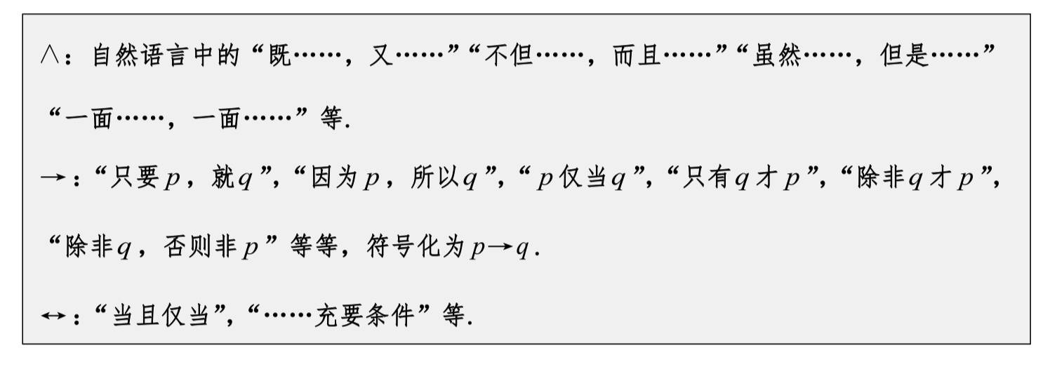
Propositions

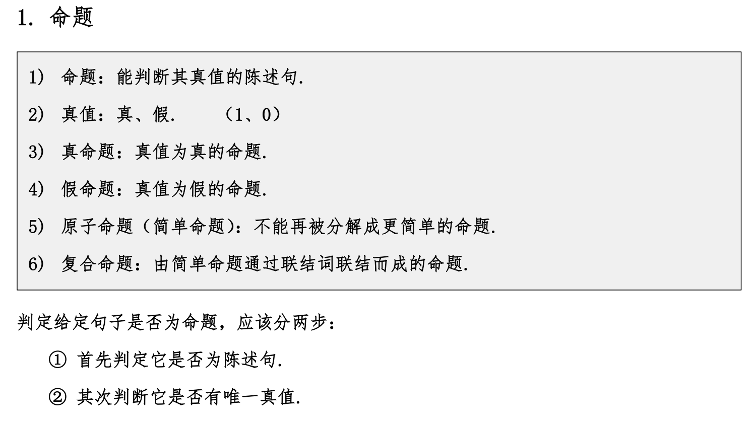
Propositional Logic

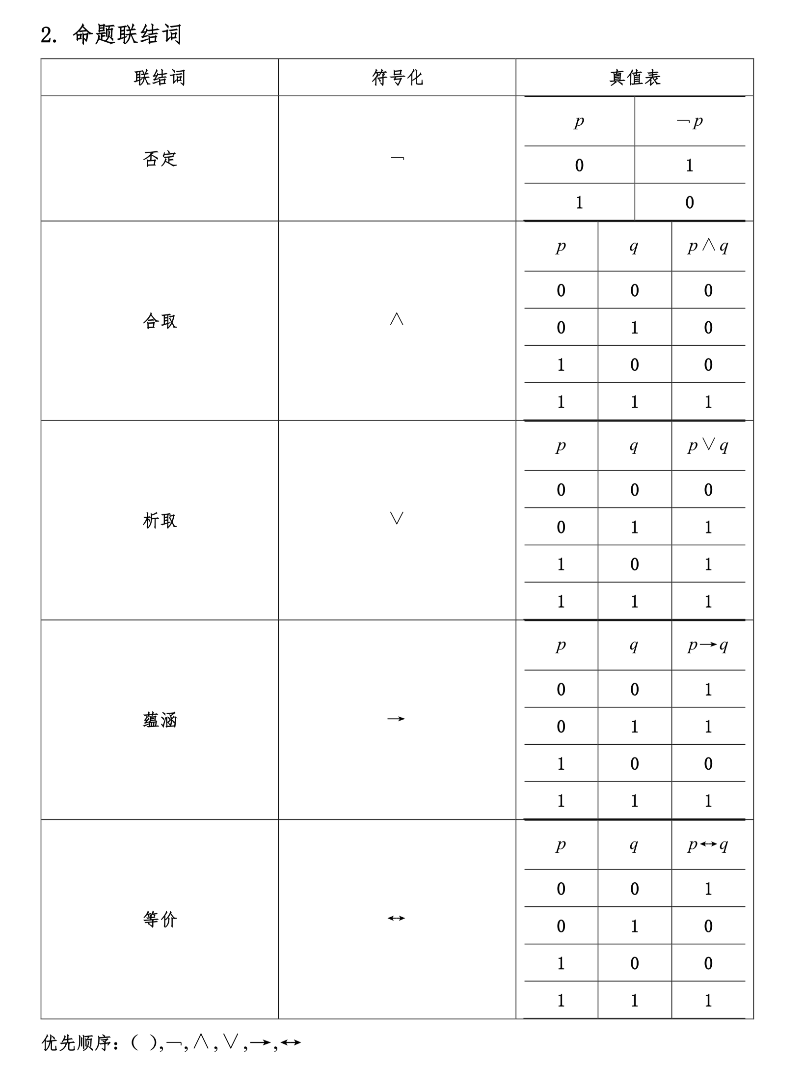
Propositional Connectives

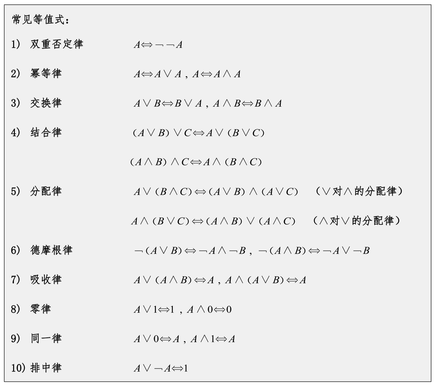
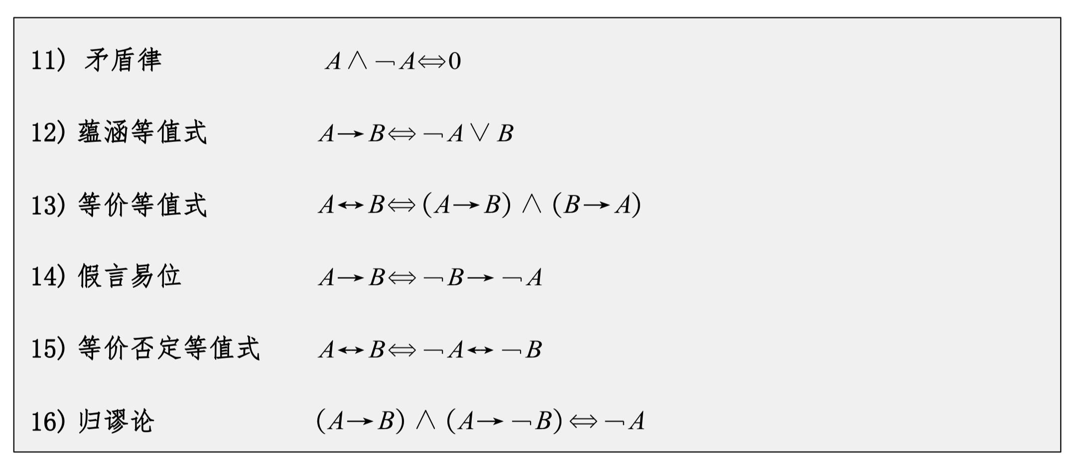
Logical Equivalences

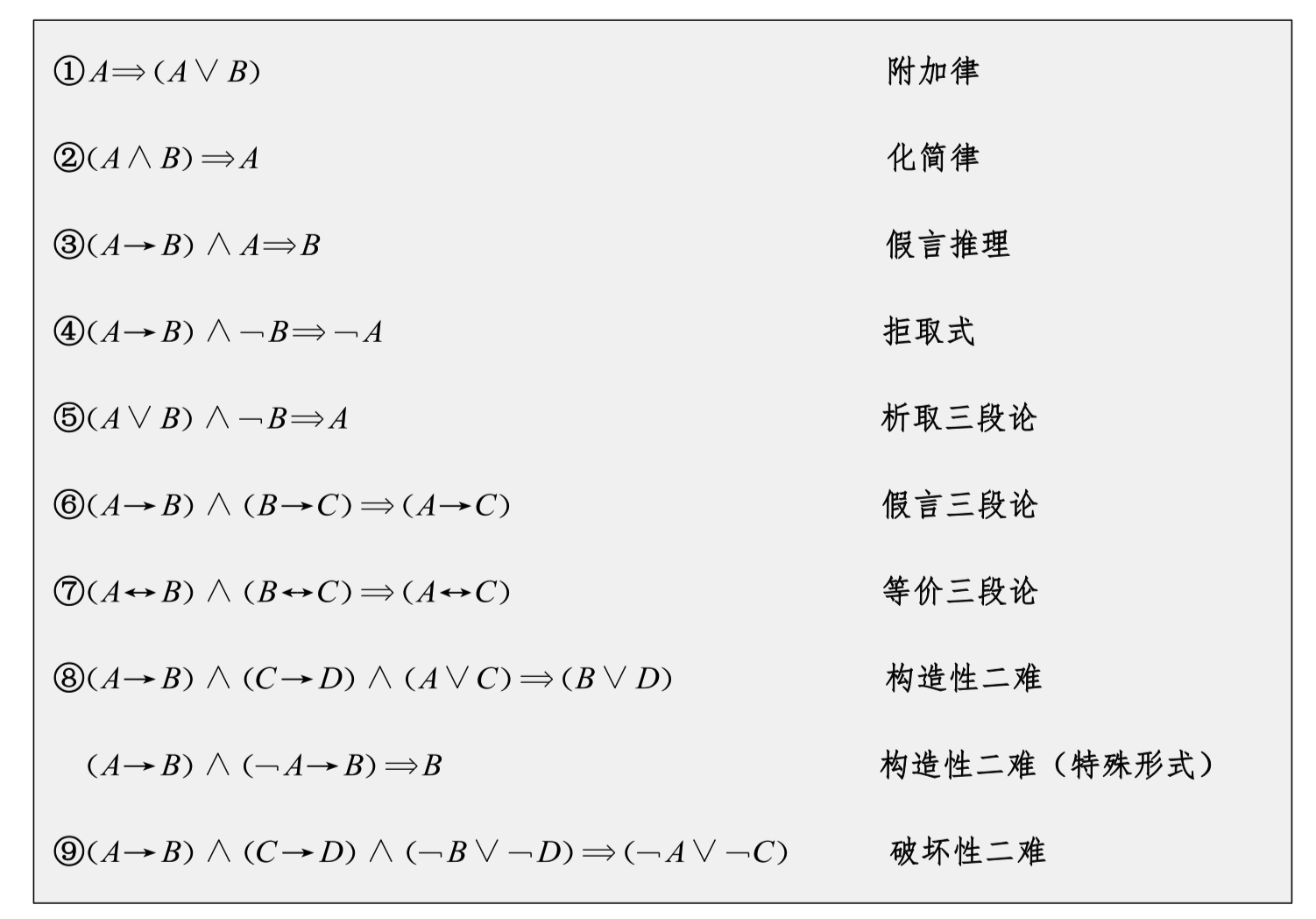
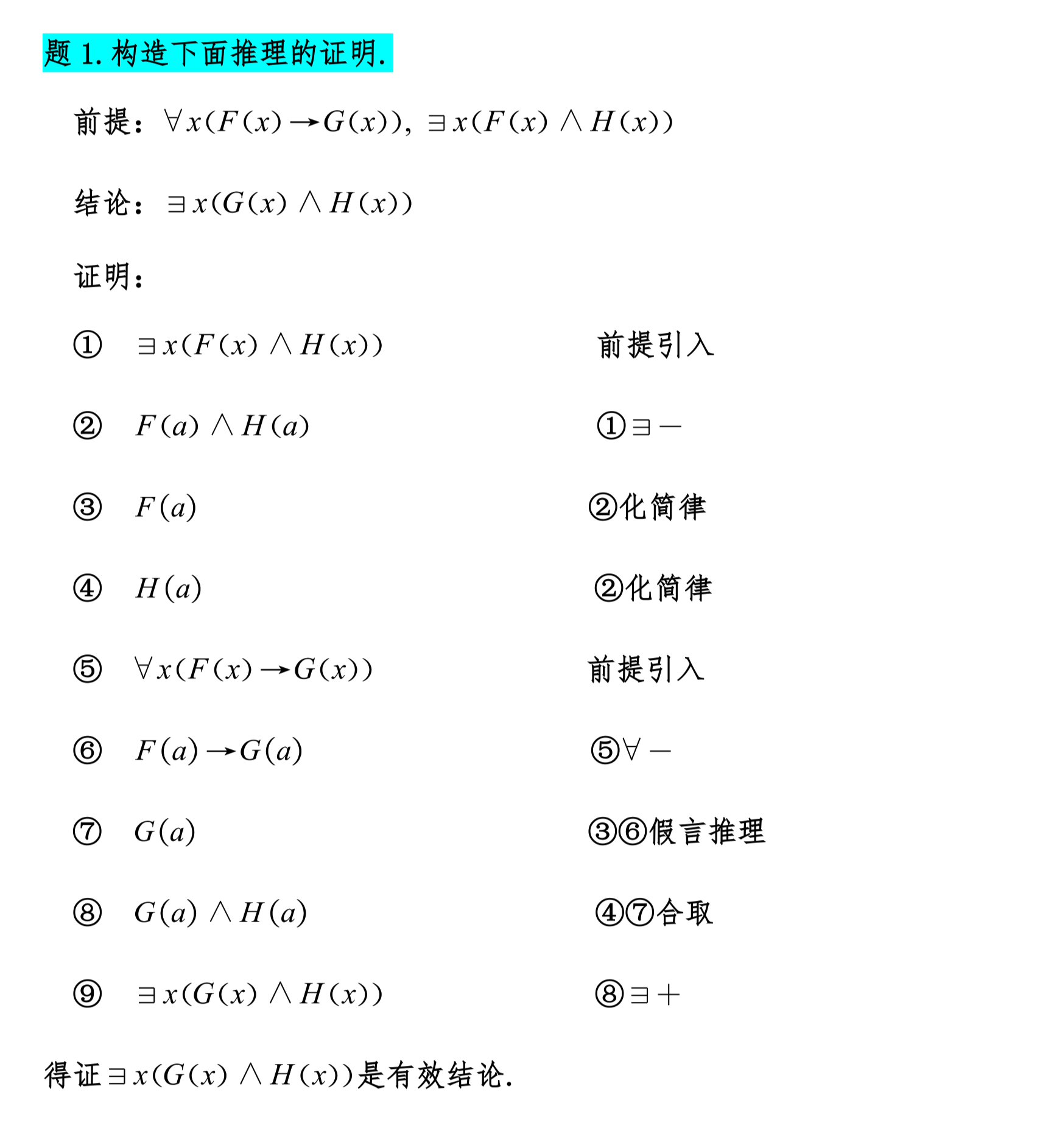
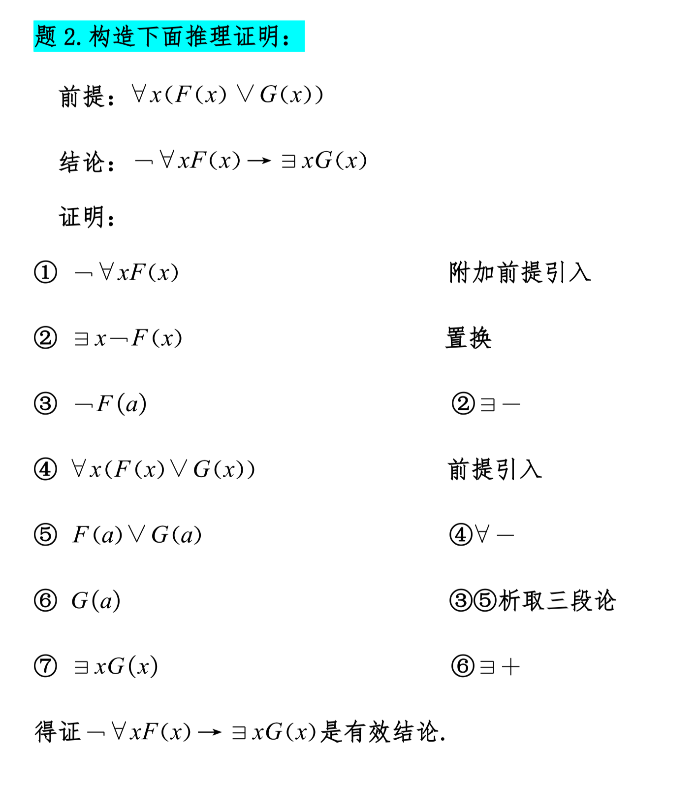
Propositional Logic Inference

Predicate Logic Equivalences

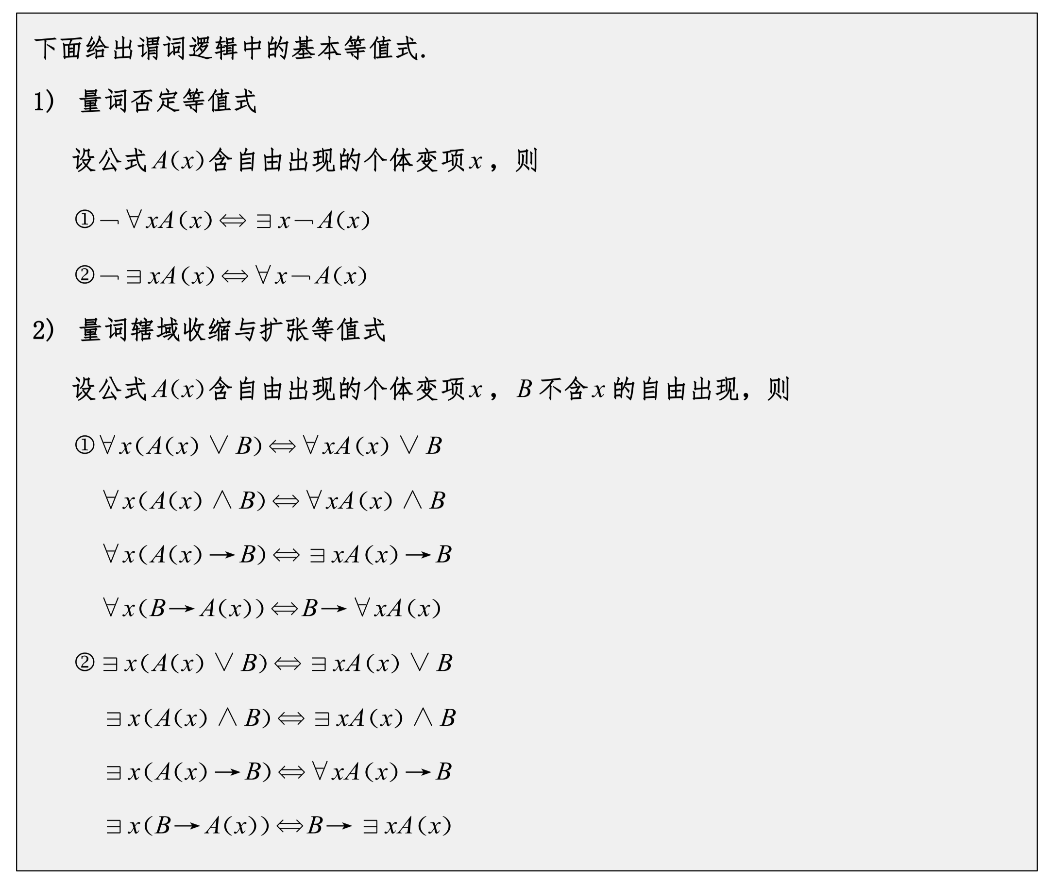
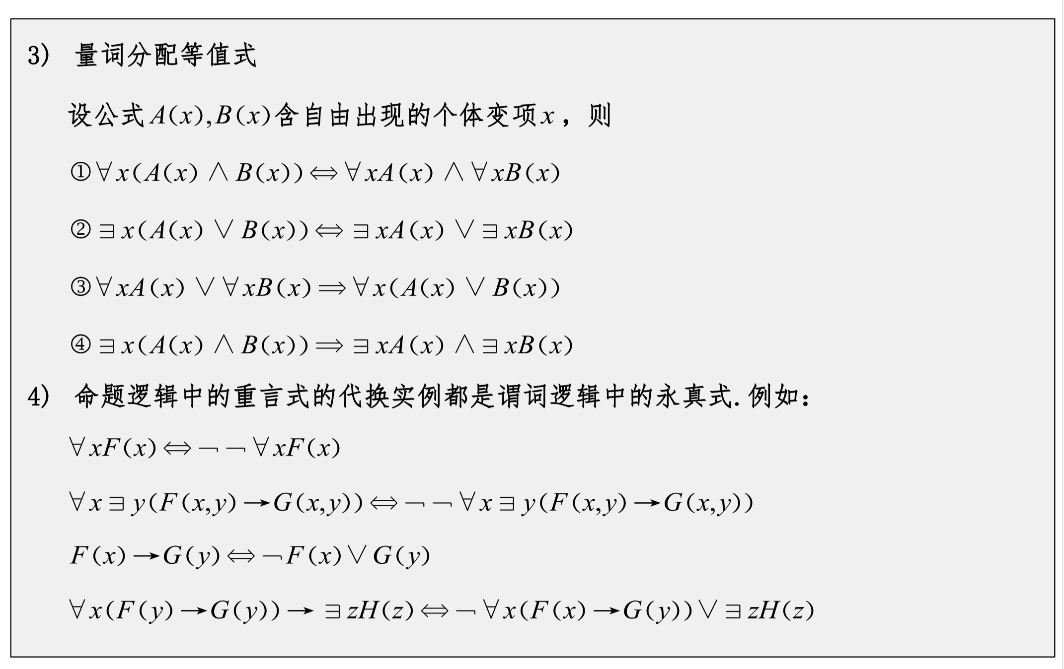
Note:

• Contraction or expansion can only be performed with disjunction or conjunction; implication must be converted to disjunction using the implication equivalence.
• Universal quantifier distributes over conjunction.
• Existential quantifier distributes over disjunction.
• Merging can be done freely, but distribution cannot be done freely.

Eliminating Quantifiers Using the Domain of Discourse

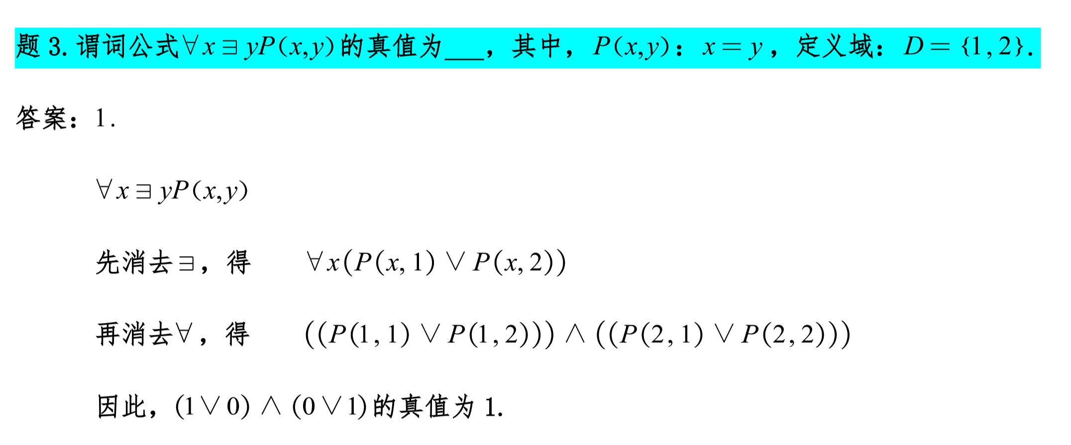
When eliminating, first eliminate the quantifier closest to the predicate.

Common Inference Laws

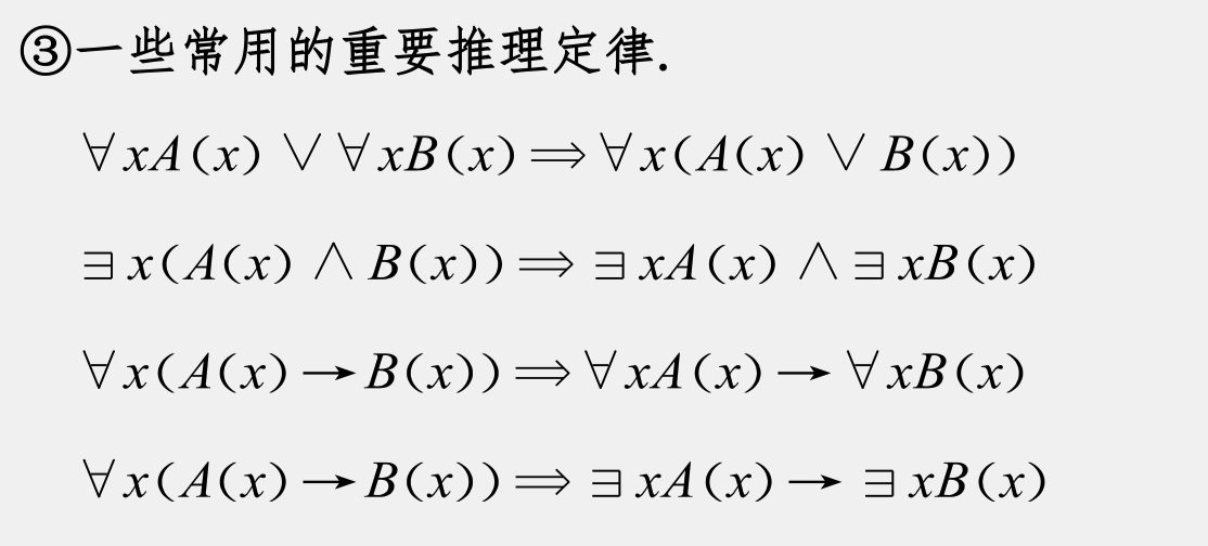
The last two expressions demonstrate the impact of using different quantifiers (universal quantifier ∀ and existential quantifier ∃) on logical propositions in logical inference.

1. First expression:

$$\forall x (A(x) \rightarrow B(x)) \implies \forall x A(x) \rightarrow \forall x B(x)$$

This expression states: if for all x, proposition A(x) implies proposition B(x), then if all x satisfy A(x), then all x satisfy B(x). In other words, if A(x) implies B(x) for every instance of x, then when A(x) holds for all x, B(x) also holds for all x.

2. Second expression: $$\forall x (A(x) \rightarrow B(x)) \implies \exists x A(x) \rightarrow \exists x B(x)$$ This expression states: if for all x, proposition A(x) implies proposition B(x), then if there exists some x satisfying A(x), then there exists some x satisfying B(x). In other words, if A(x) implies B(x) for every instance of x, then if at least one x makes A(x) hold, at least one x makes B(x) hold.

The difference between these two expressions lies in the quantifiers in the conclusion:

• The conclusion of the first expression involves the universal quantifier ∀, meaning all x must satisfy a certain condition.
• The conclusion of the second expression involves the existential quantifier ∃, meaning at least one x satisfies a certain condition.

Although these two expressions have the same premise, the different quantifiers in the conclusion lead to different meanings. In logical inference, changes in quantifiers significantly affect the meaning and inference process of propositions.

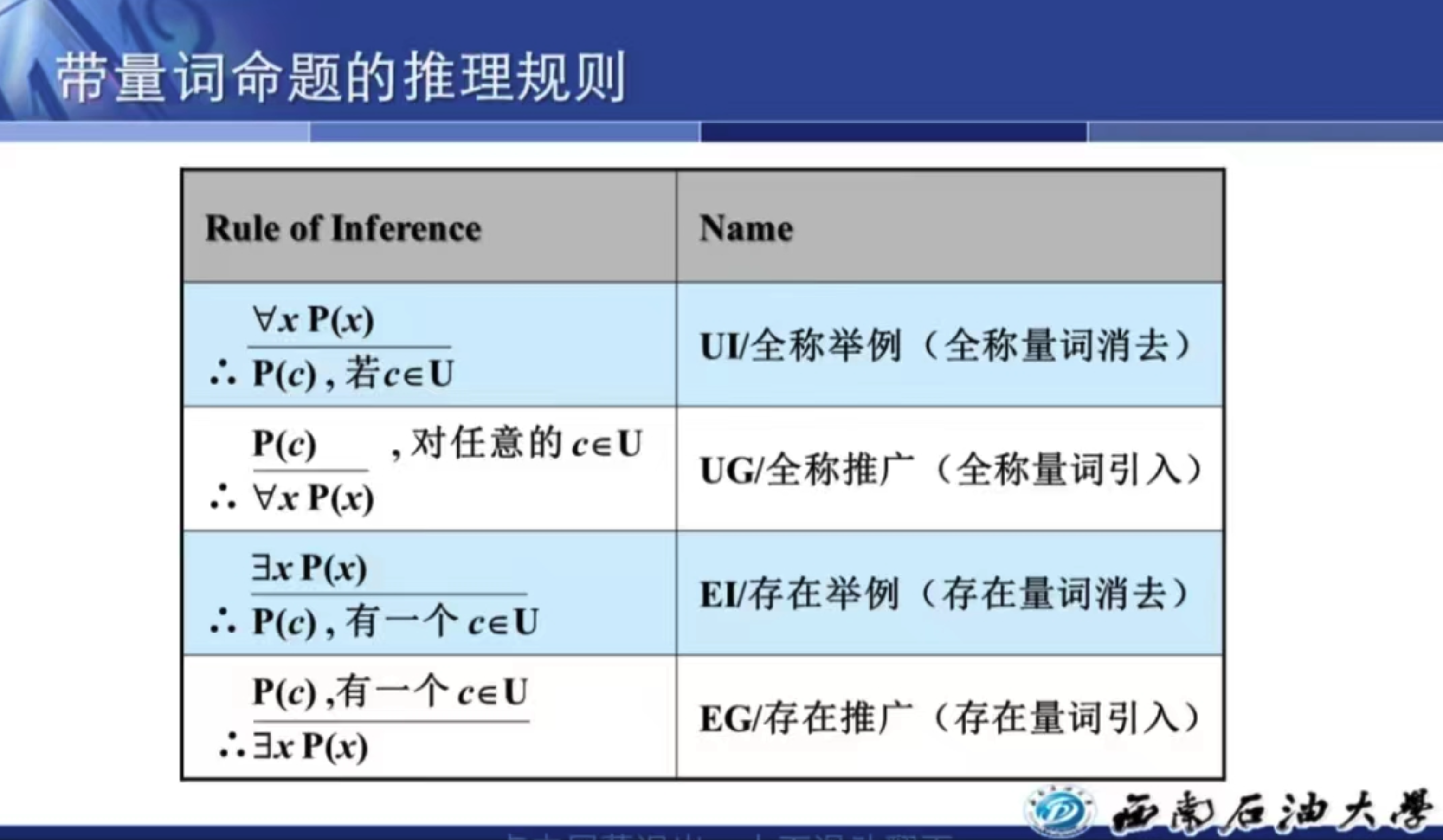
Quantifier Elimination and Introduction

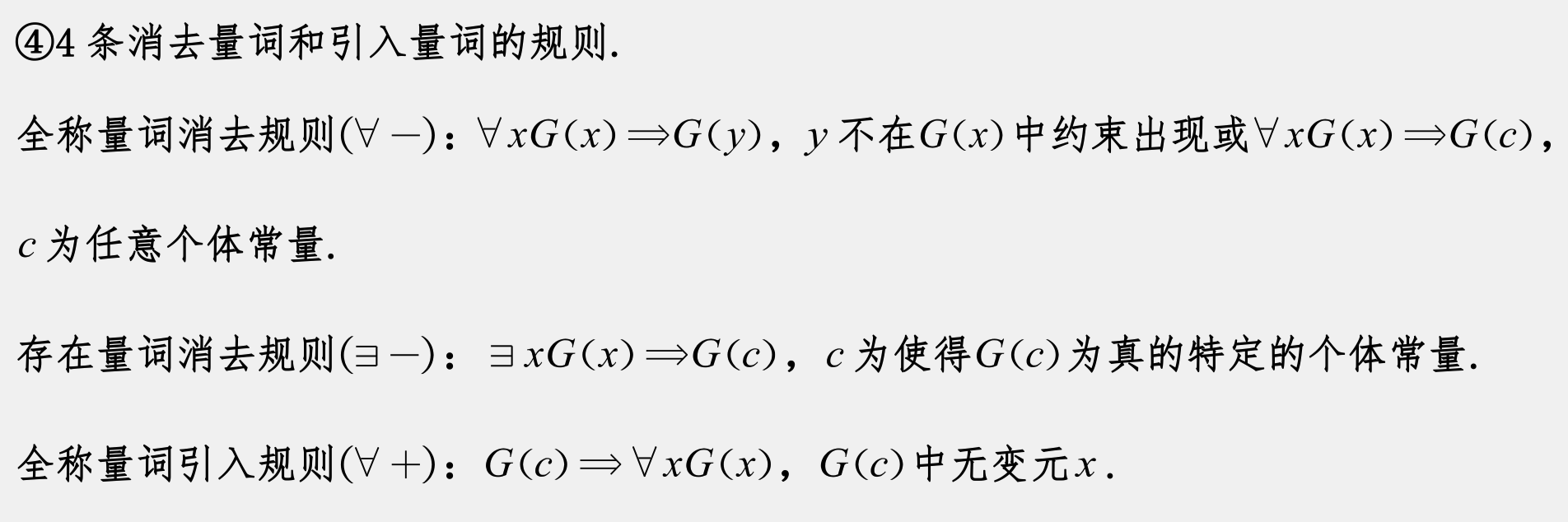
Existential Elimination

The existential elimination rule allows us to derive a quantifier-free proposition from an existentially quantified proposition. Formally, if we know that ∃x P(x) is true, then we can introduce a new constant c such that P(c) is true.

Rule form:

$$\frac{\exists x \, P(x)}{P(c)}$$

Notes:

• The constant c must be a new symbol, i.e., it has not appeared before in the current inference process.

Example: Suppose we know ∃x (x > 0), then we can introduce a new constant c such that c > 0.

Existential Introduction

The existential introduction rule allows us to derive an existentially quantified proposition from a specific proposition. Formally, if we know P(c) is true, then we can derive ∃x P(x).

Rule form:

$$\frac{P(c)}{\exists x \, P(x)}$$

Notes:

• The constant c can be any constant, not necessarily a new symbol.

Example: Suppose we know c > 0, then we can derive ∃x (x > 0).

Universal Elimination

The universal elimination rule allows us to derive a specific proposition from a universally quantified proposition. Formally, if we know ∀x P(x) is true, then for any object a, P(a) is also true.

Rule form:

$$\frac{\forall x \, P(x)}{P(a)}$$

Notes:

• The object a can be any object, including variables, constants, or function terms.

Example: Suppose we know ∀x (x ≥ 0), then for any a, we can derive a ≥ 0.

Universal Introduction

The universal introduction rule allows us to derive a universally quantified proposition from a specific proposition. Formally, if for any object a, P(a) is true, then we can derive ∀x P(x).

Rule form:

$$\frac{P(a) \text{ for arbitrary } a}{\forall x \, P(x)}$$

Notes:

• The object a must be arbitrary, meaning it cannot have any specific properties or restrictions in the inference process.

Example: Suppose we can prove that for any a, a² ≥ 0, then we can derive ∀x (x² ≥ 0).

Additional Premise Introduction

Sets

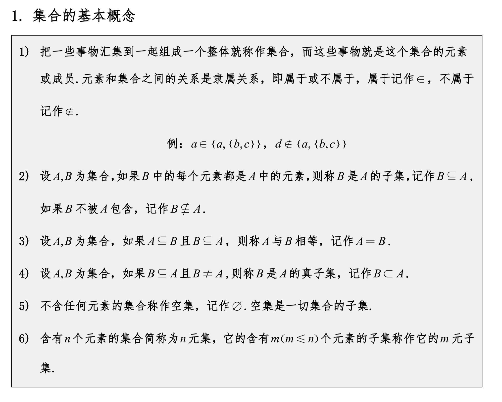
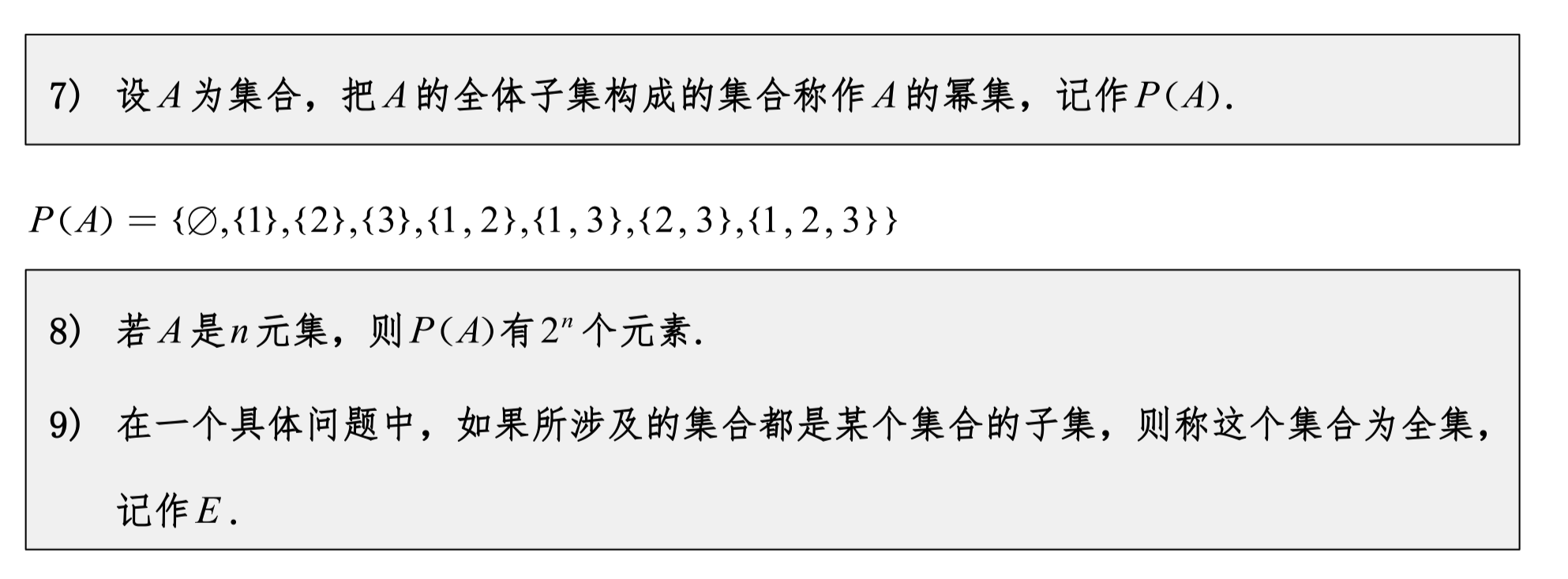
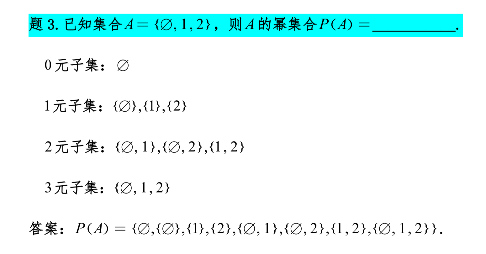
The empty set explicitly written in a set can be treated as just a symbol.

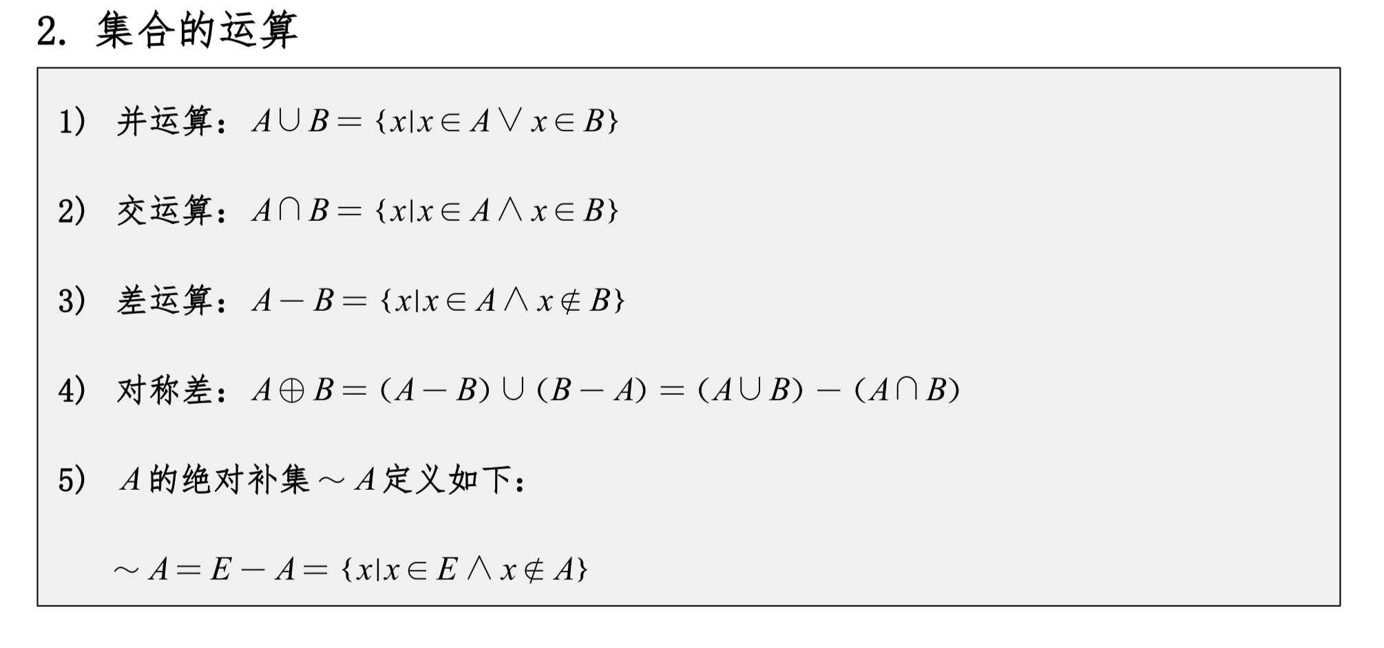
Set Operations

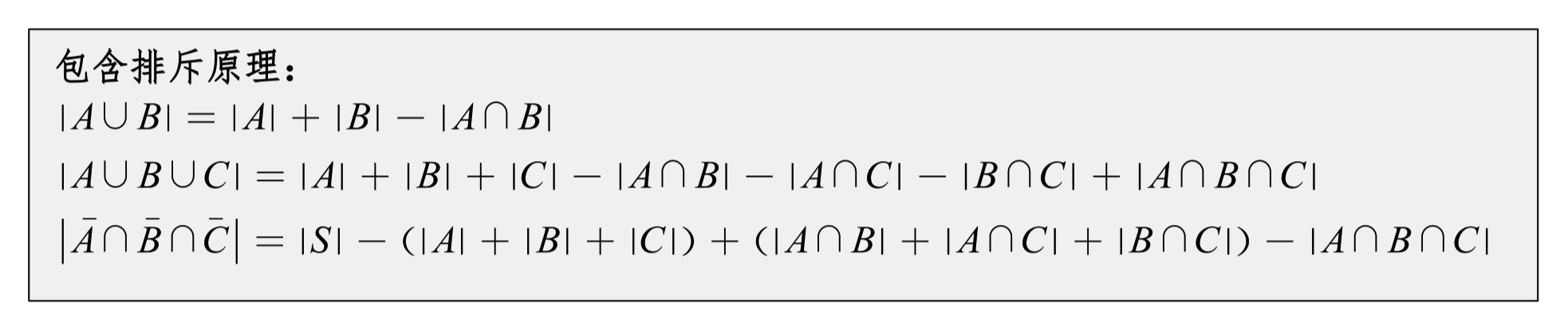
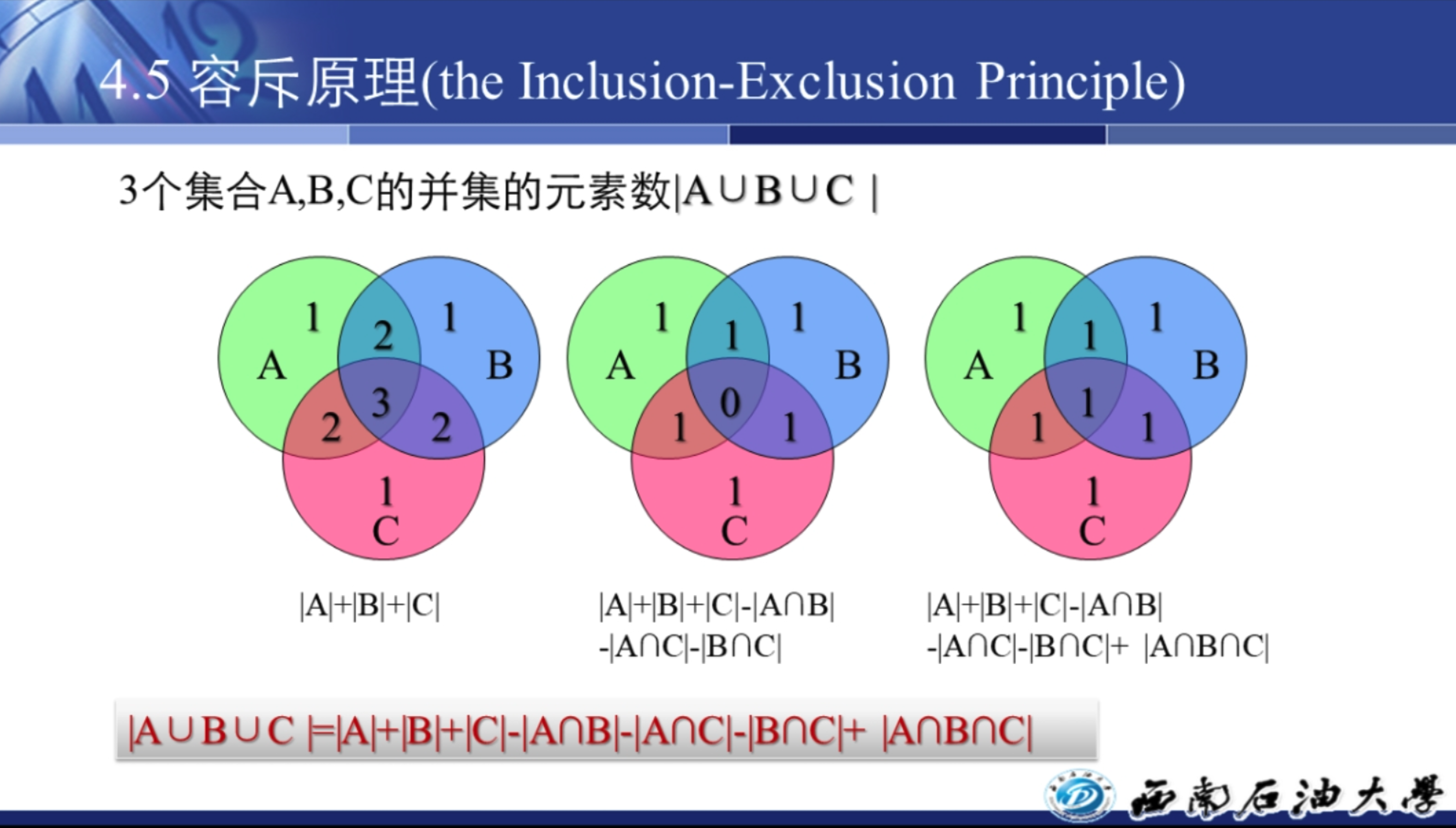
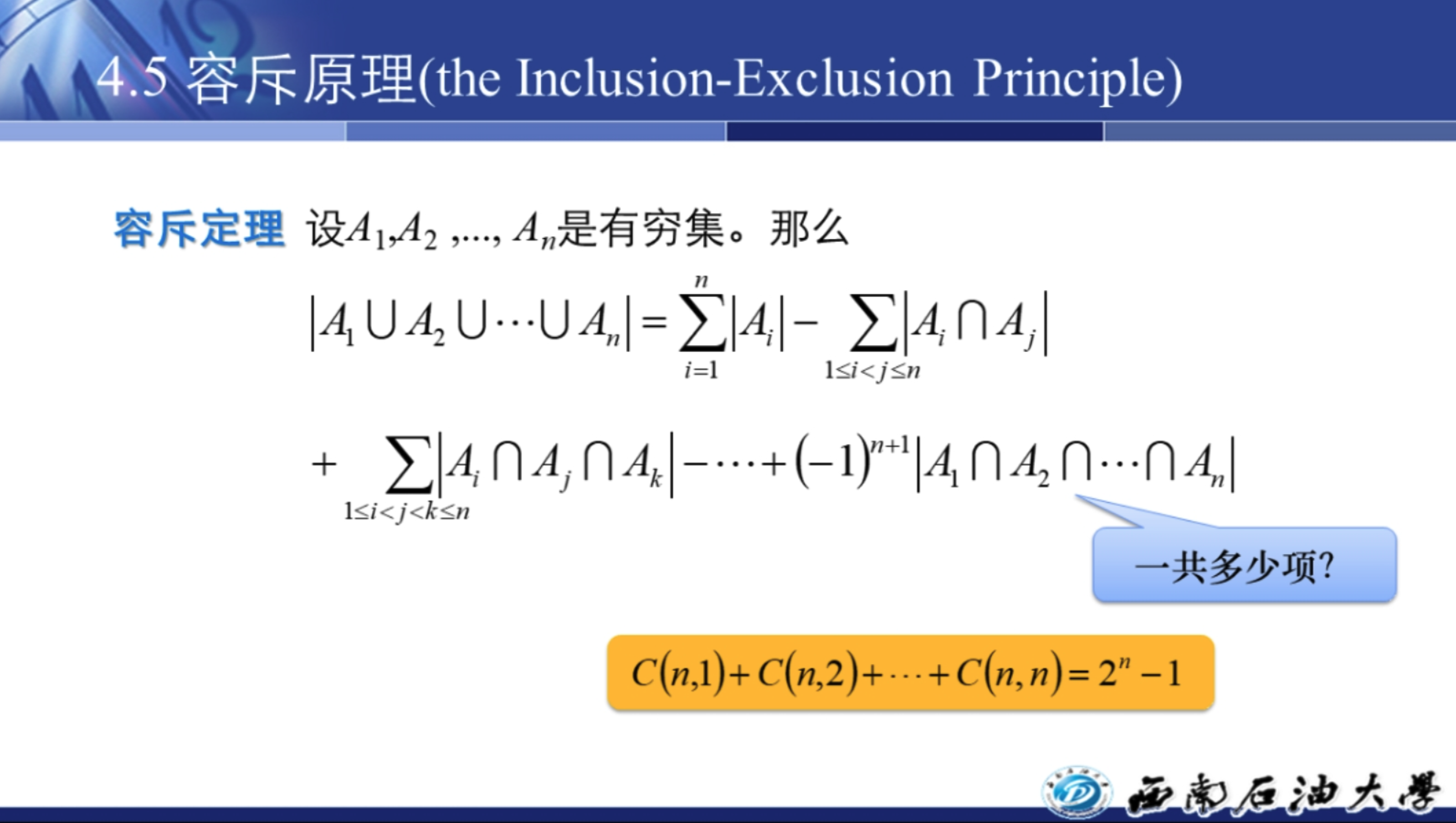
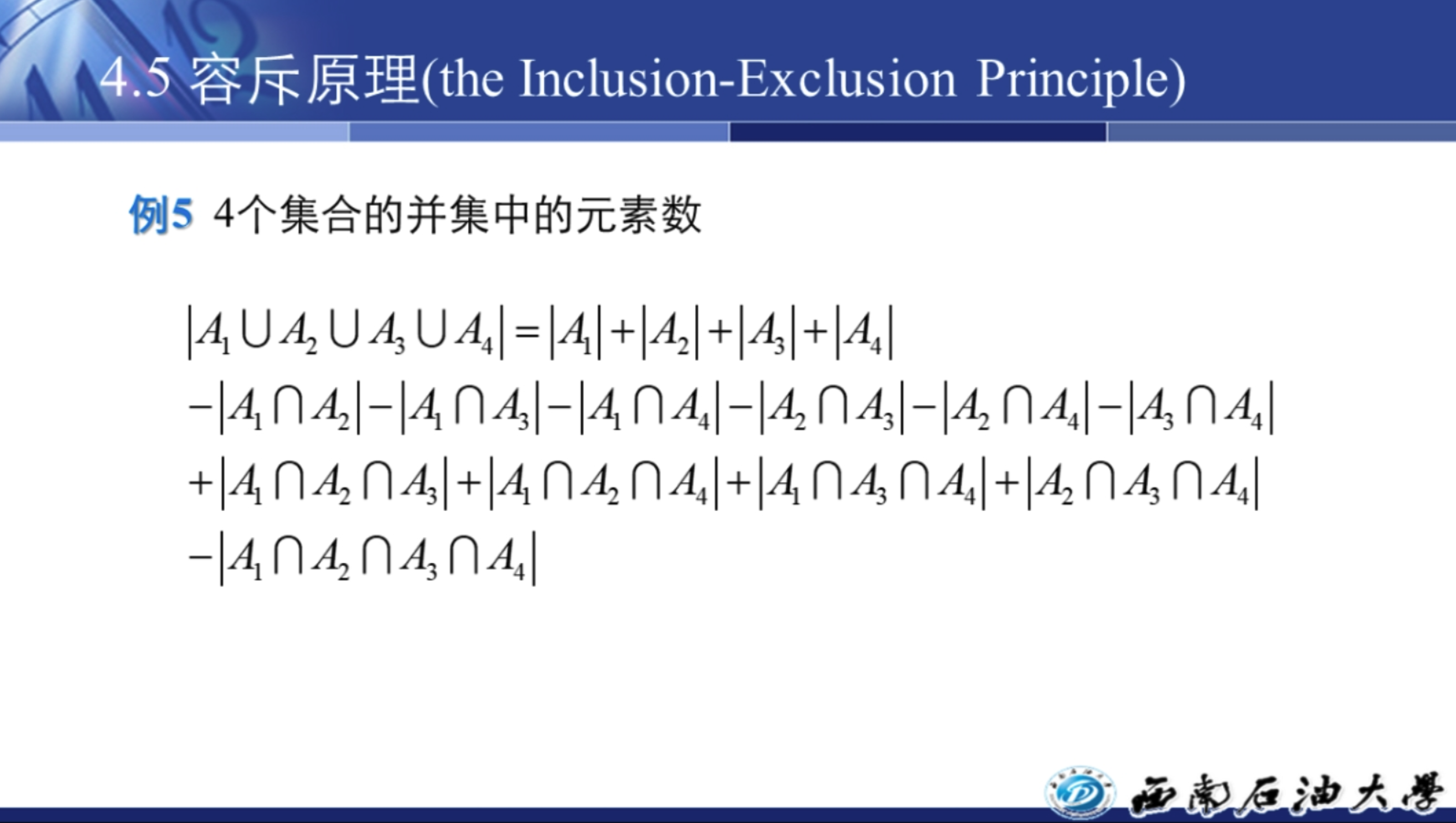
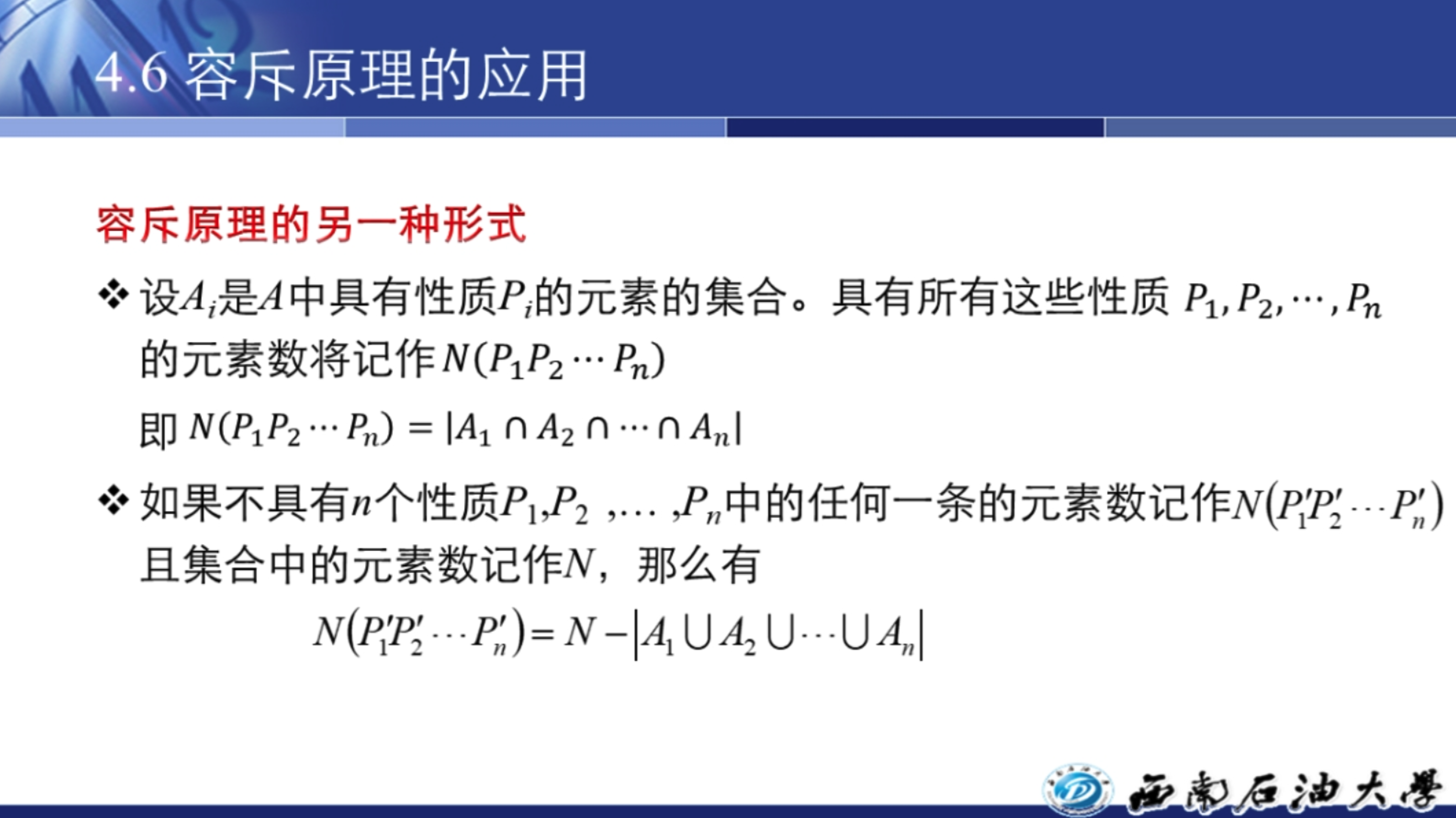
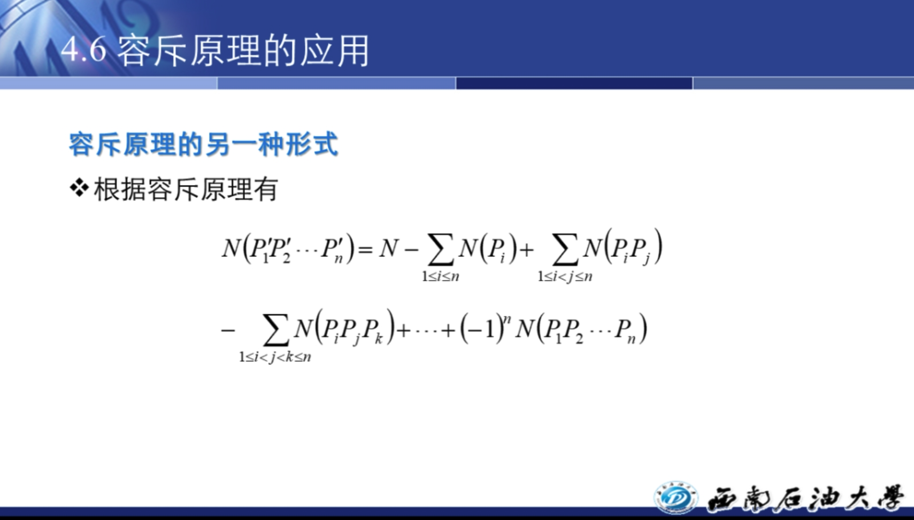
Inclusion-Exclusion Principle

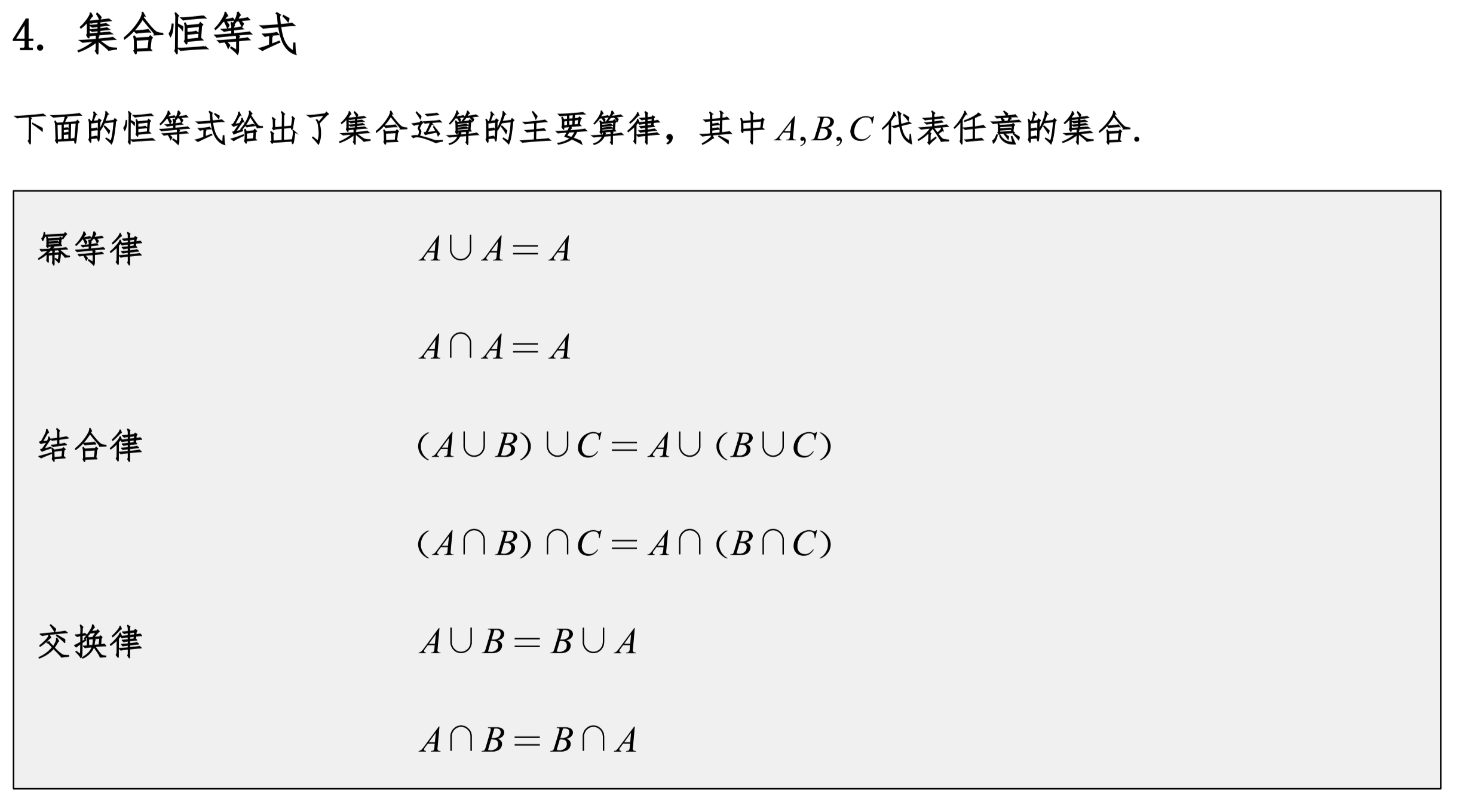
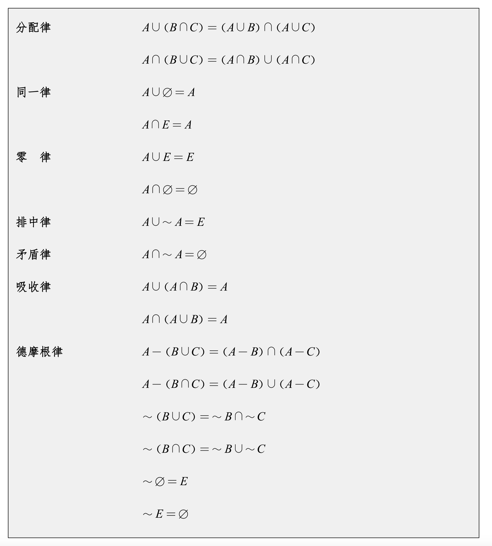
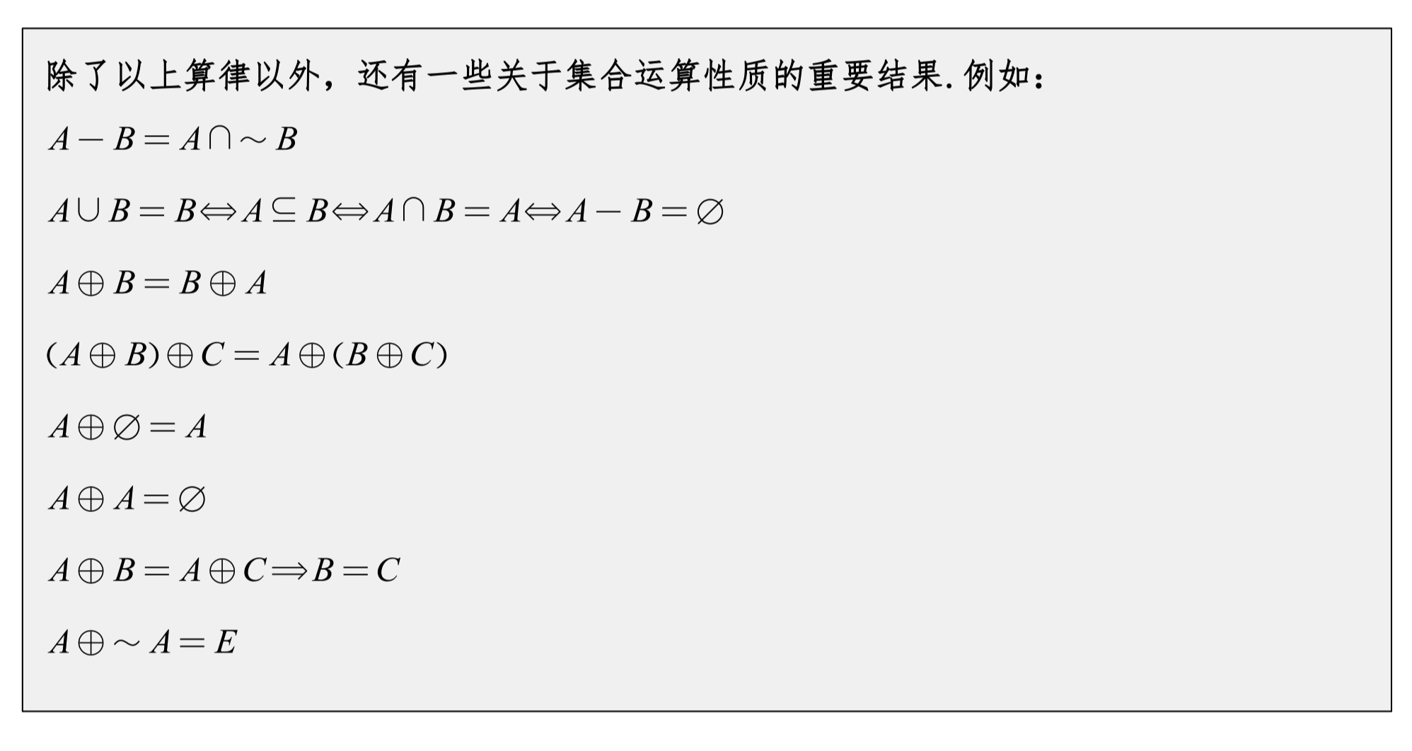
Set Identities

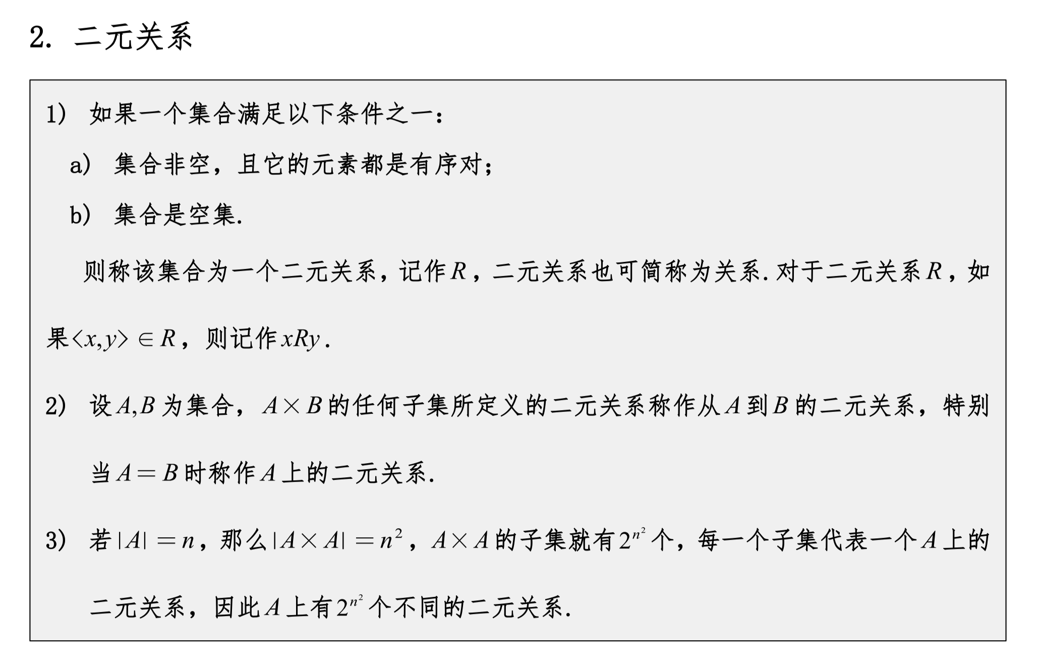
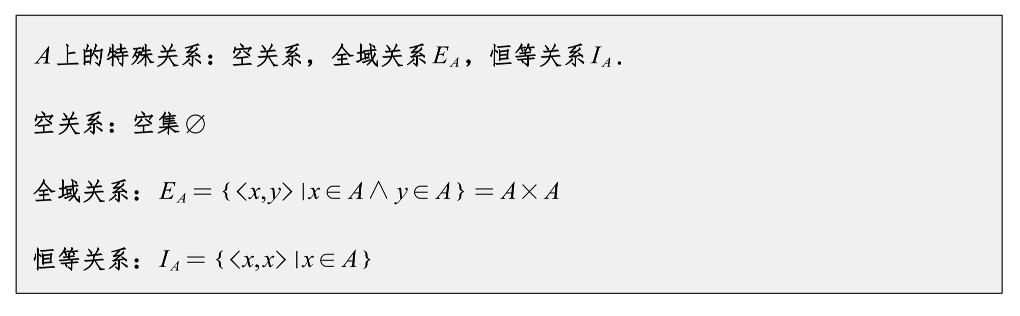
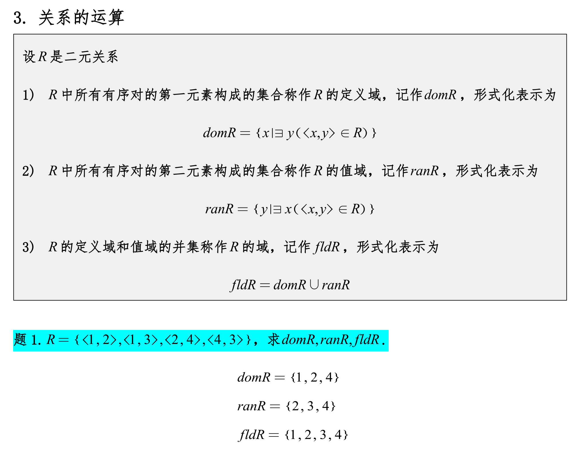
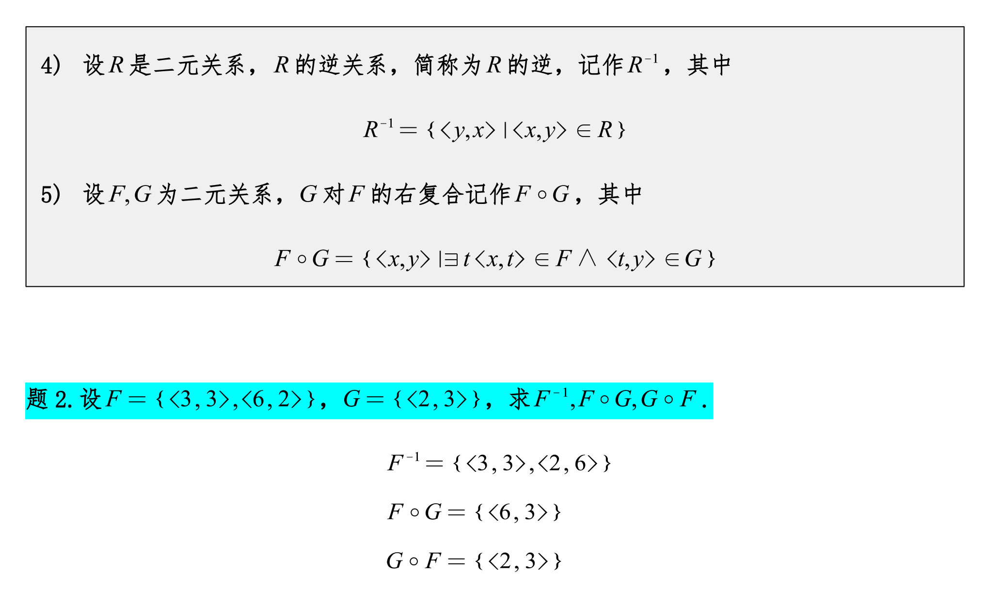
Binary Relations

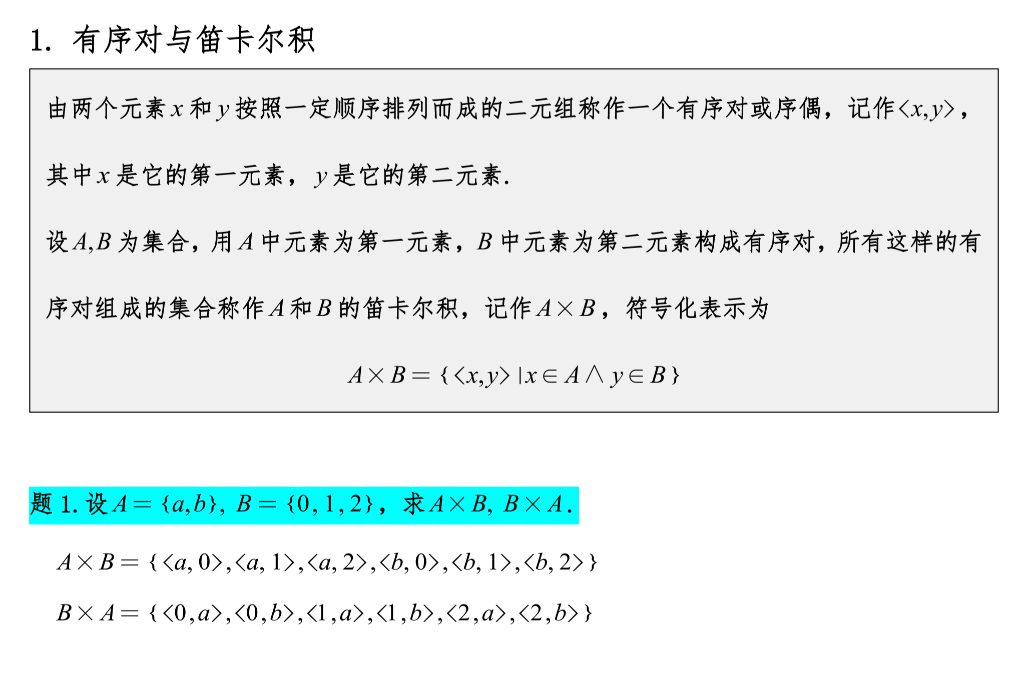
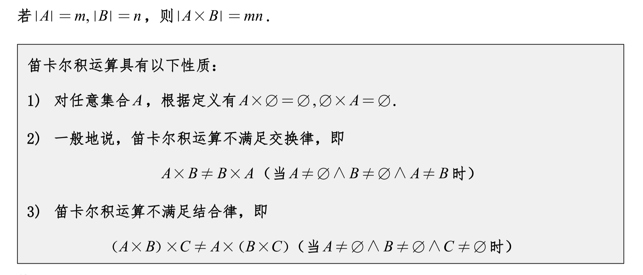
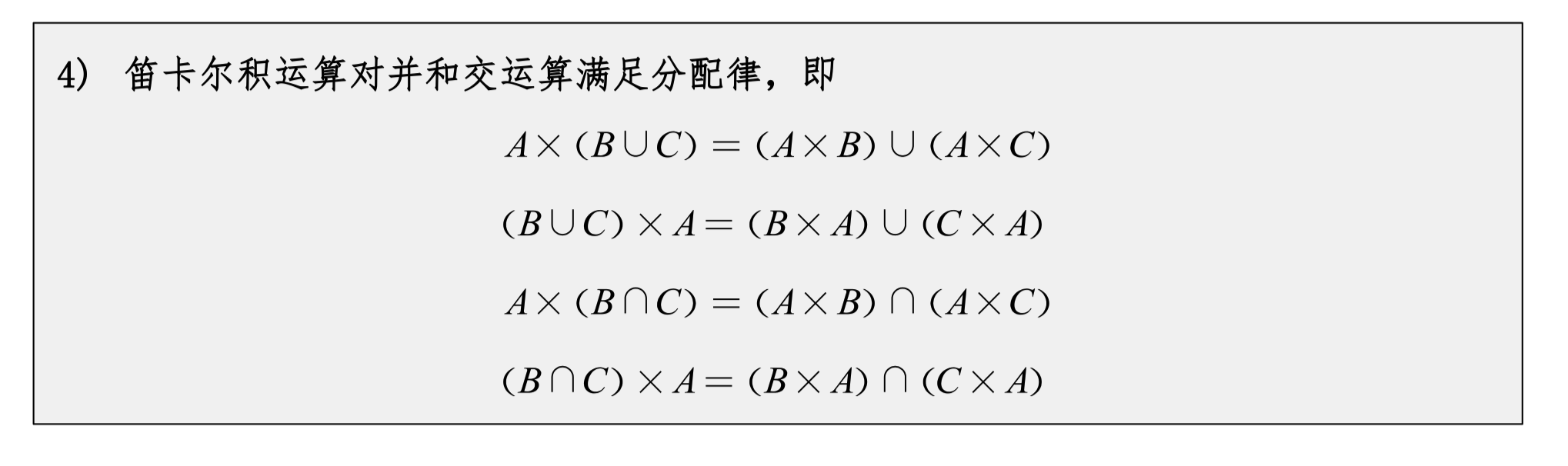
The Cartesian product does not satisfy the commutative property.

Binary Relations

Operations on Relations

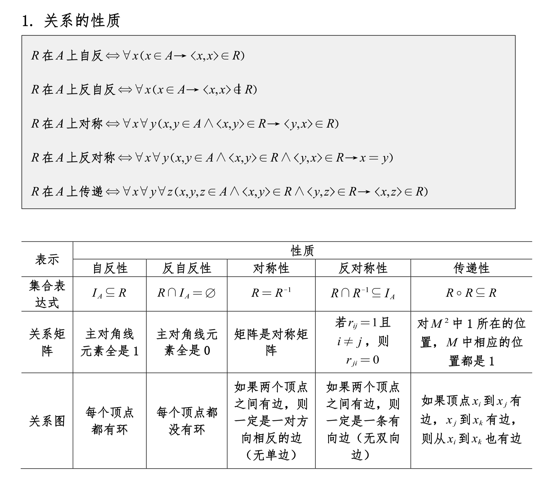
Properties of Relations

What is the transitive closure of $\{(a,b),(b,c)\}$?

Given the relation $R = \{(a, b), (b, c)\}$, we need to find its transitive closure. The transitive closure is obtained by adding all relation pairs that can be derived through transitivity, making the relation transitive.

The transitive closure R⁺ is defined as: if (x, y) ∈ R⁺ and (y, z) ∈ R⁺, then (x, z) ∈ R⁺.

First, the elements in the original relation R are:

$$R = \{(a, b), (b, c)\}$$

Next, check for relation pairs obtainable through transitivity:

1. (a, b) ∈ R and (b, c) ∈ R, so by transitivity (a, c) must also be in the transitive closure.

Therefore, the transitive closure R⁺ is:

$$R^+ = \{(a, b), (b, c), (a, c)\}$$

So, the transitive closure of relation $R = \{(a, b), (b, c)\}$ is:

$$R^+ = \{(a, b), (b, c), (a, c)\}$$

Let set A have 3 elements. The number of equivalence relations that can be defined on A is ( ).

An equivalence relation partitions a set into several disjoint subsets. The number of equivalence relations equals the number of all possible partitions of set A, known as the Bell number.

For set $A = \{a, b, c\}$, calculate its Bell number.

We examine all possible partitions of set $\{1, 2, 3\}$ in order:

1. One subset: $\{\{a, b, c\}\}$
2. Two subsets: $\{\{a\}, \{b, c\}\}$, $\{\{b\}, \{a, c\}\}$, $\{\{c\}, \{a, b\}\}$
3. Three subsets: $\{\{a\}, \{b\}, \{c\}\}$

The specific calculation method is as follows:

• B₁ = 1 (a set with 1 element has only one partition)
• B₂ = 2 (a set with 2 elements has two partitions: one set or two singleton sets)
• B₃ is what needs to be calculated.

Using the Bell number recurrence formula: $B_{n+1} = \sum_{k=0}^n \binom{n}{k} B_k$

Specifically calculating B₃: $B_3 = \sum_{k=0}^2 \binom{2}{k} B_k$

Calculation process: $B_3 = \binom{2}{0} B_0 + \binom{2}{1} B_1 + \binom{2}{2} B_2$ $B_3 = 1 \cdot 1 + 2 \cdot 1 + 1 \cdot 2$ $B_3 = 1 + 2 + 2$ $B_3 = 5$

Therefore, the number of equivalence relations that can be defined on set A is 5.

Answer: 5

In mathematics, ceiling and floor functions use different symbols.

1. Ceiling function:

   • Symbol: ⌈x⌉
   • Meaning: Rounds the value x up to the nearest integer. If x is already an integer, the result is x itself. For example: ⌈3.2⌉ = 4, ⌈-2.7⌉ = -2.

2. Floor function:

   • Symbol: ⌊x⌋
   • Meaning: Rounds the value x down to the nearest integer. If x is already an integer, the result is x itself. For example: ⌊3.8⌋ = 3, ⌊-2.3⌋ = -3.

These two symbols are used to represent rounding up or down and are widely used in mathematics and computer science.

Note

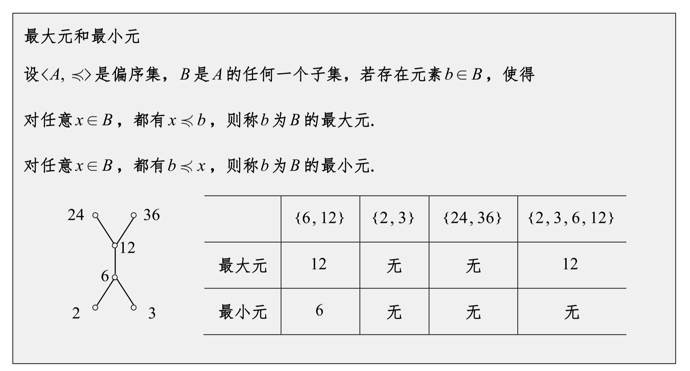
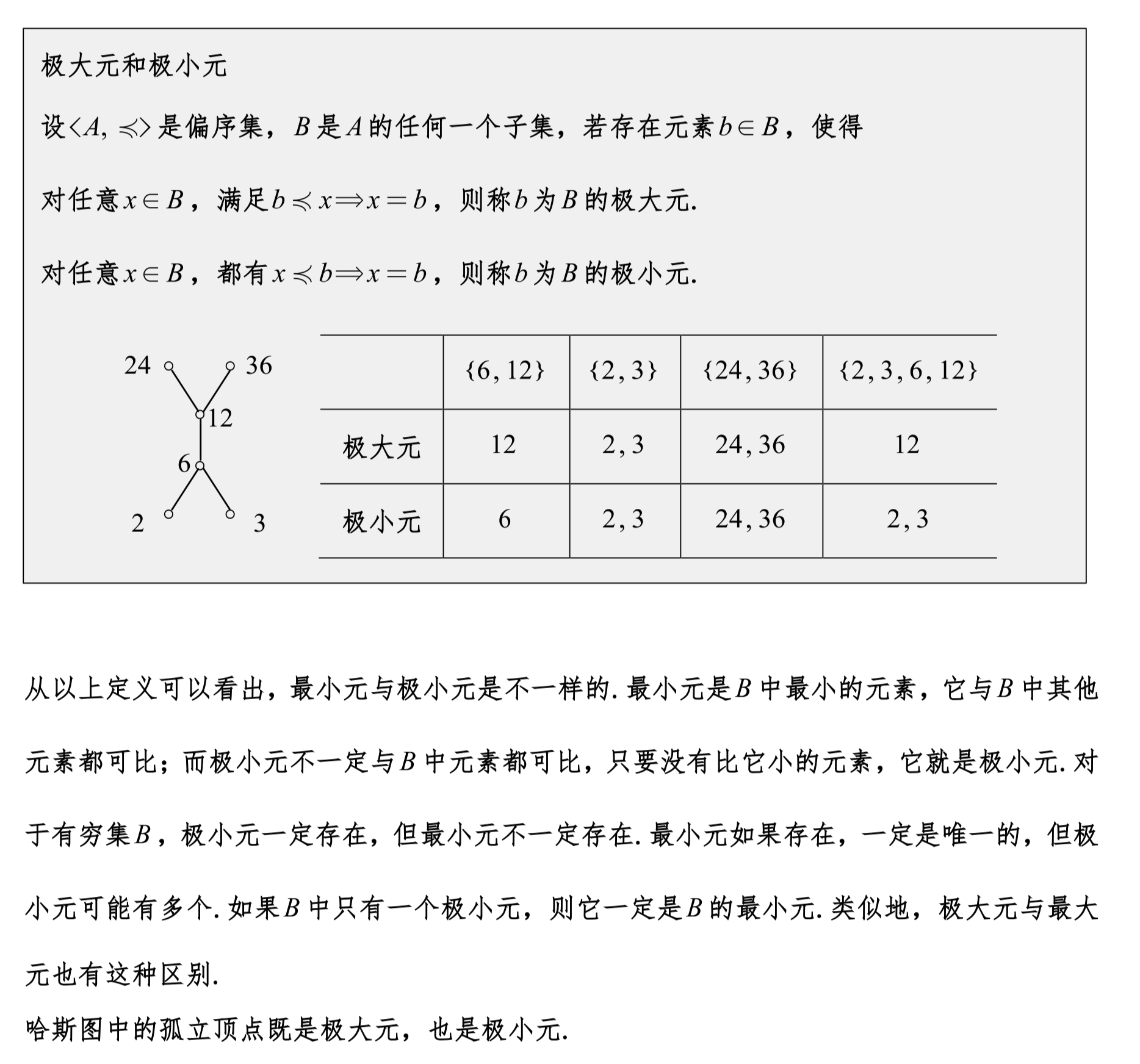
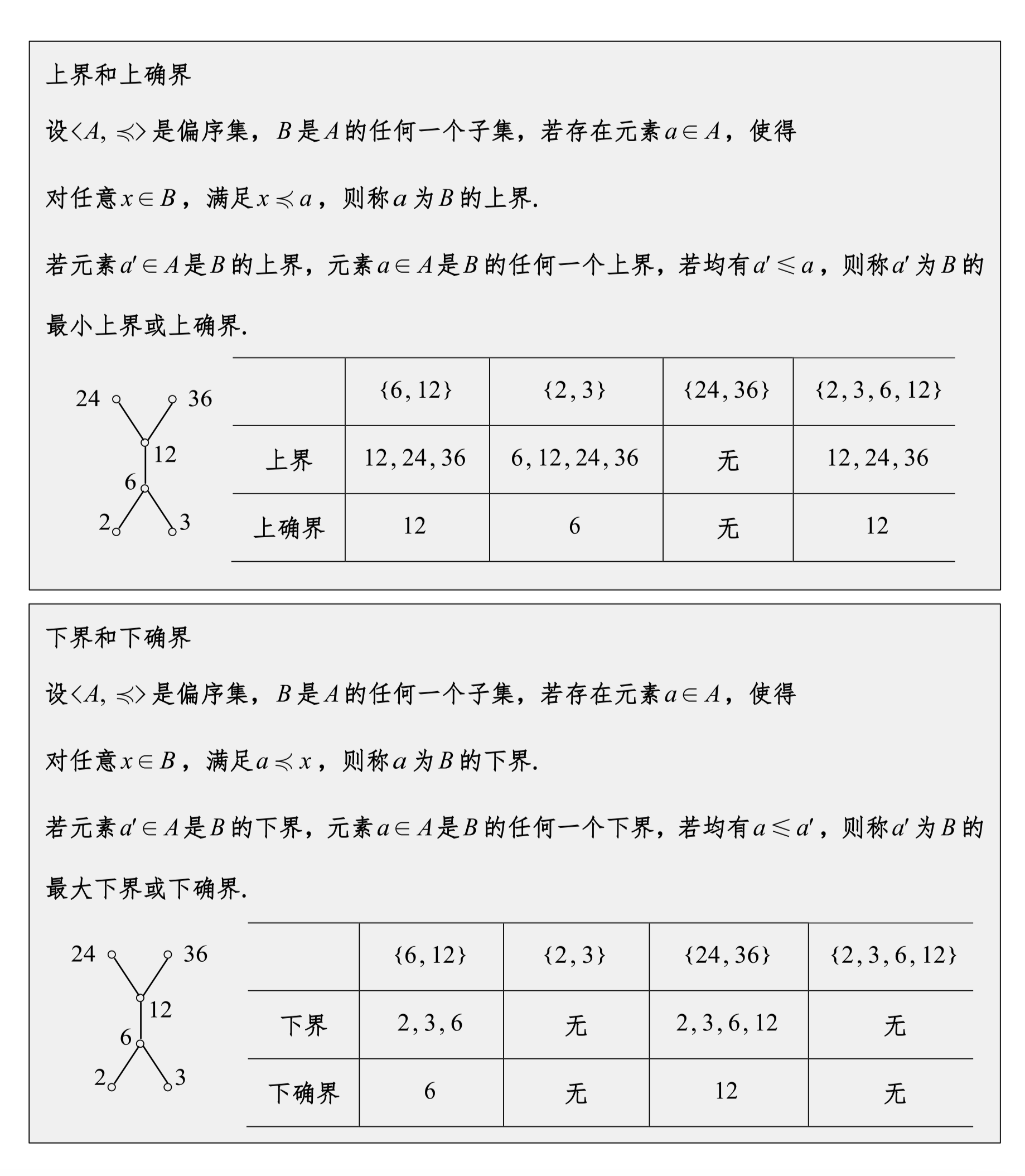
Maxima and minima are searched within the given set.

Bounds are searched within the entire Hasse diagram.

Incomparable elements do not have maxima/minima, but may have maximal/minimal elements.

Both concepts include "greater than or equal to" and "less than or equal to" — never forget "equal to."

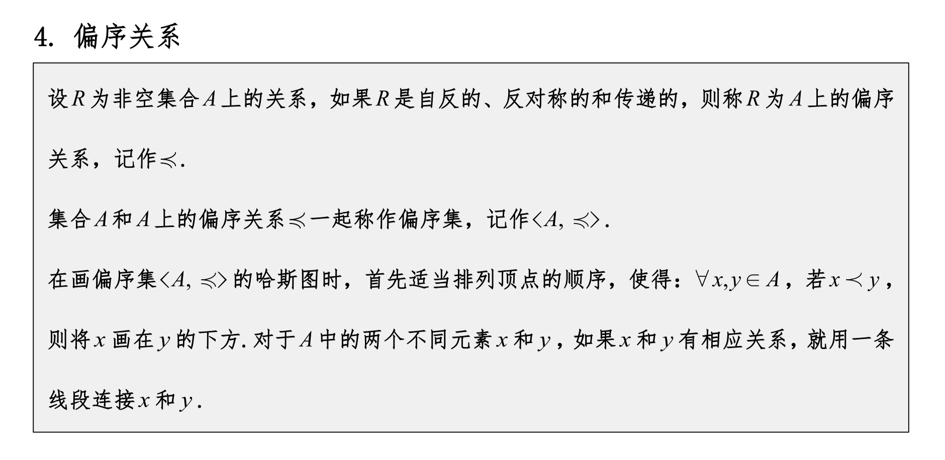
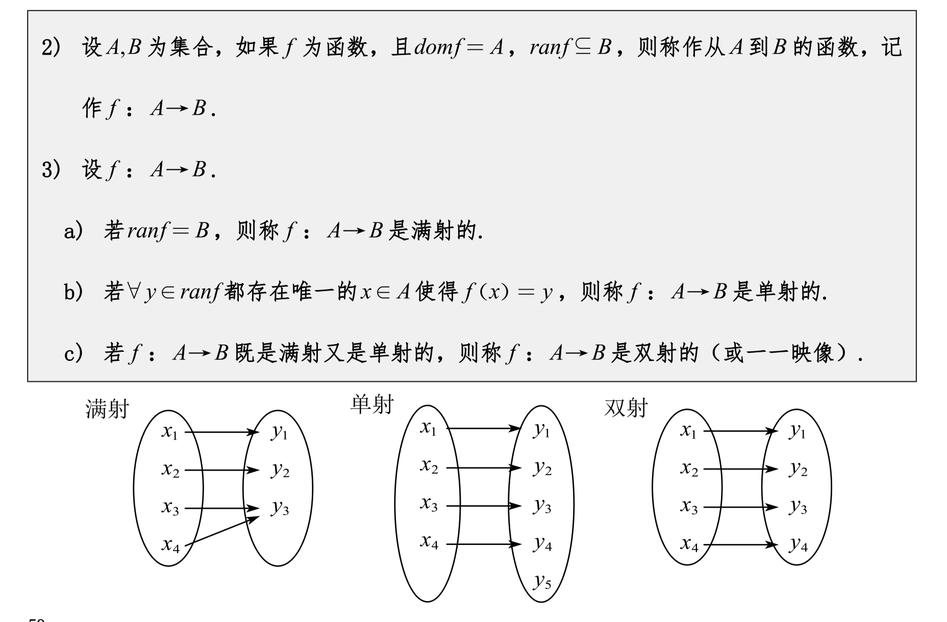
Functions

Graphs

Handshaking Theorem

Degree Sum Theorem

First, we need to understand some basic concepts:

• Degree of a vertex: The degree of a vertex is the number of edges connected to that vertex.
• Degree sum of a graph: The sum of the degrees of all vertices in a graph equals twice the number of edges in the graph.

The degree sum theorem can be stated as: $\sum_{v \in V} \deg(v) = 2|E|$

where deg(v) represents the degree of vertex v, V is the vertex set, and E is the edge set.

Properties of Odd and Even Numbers

• Odd plus odd equals even.
• Odd plus even equals odd.
• Even plus even equals even.

Proving the Number of Odd-Degree Vertices Is Even

According to the degree sum theorem, the sum of all vertex degrees in a graph is an even number 2|E|.

Now, consider dividing all vertex degrees into two categories: odd-degree vertices and even-degree vertices.

Let the graph have k odd-degree vertices. Since the sum of degrees of even-degree vertices is obviously even, we can use S_odd and S_even to denote the sum of degrees of odd-degree and even-degree vertices respectively. Then: $S_{\text{odd}} + S_{\text{even}} = 2|E|$

where S_even is even (because the sum of an even number of even numbers is even), and 2|E| is also even.

Therefore, S_odd must also be even, because even minus even is still even.

Considering that the sum of odd numbers is odd only when an odd number of odd numbers are added, and even when an even number of odd numbers are added, S_odd being even means the number of odd-degree vertices k must be even.

Conclusion

The number of odd-degree vertices in any graph is always even. This is because the sum of all vertex degrees in a graph is even, and only the sum of an even number of odd numbers is even, so an odd number of odd numbers cannot sum to an even number.

Degree Sequence

Method to Determine if a Sequence Can Be a Degree Sequence

The total degree must be even.

The number of odd-degree vertices must be even.

The maximum degree must be less than n-1; in a simple undirected graph, a vertex can be connected to at most n-1 other vertices.

Complete Undirected Graph

Connectivity

If there exists a path from u to v, then u is reachable from v. Note that the existence of a path is sufficient.

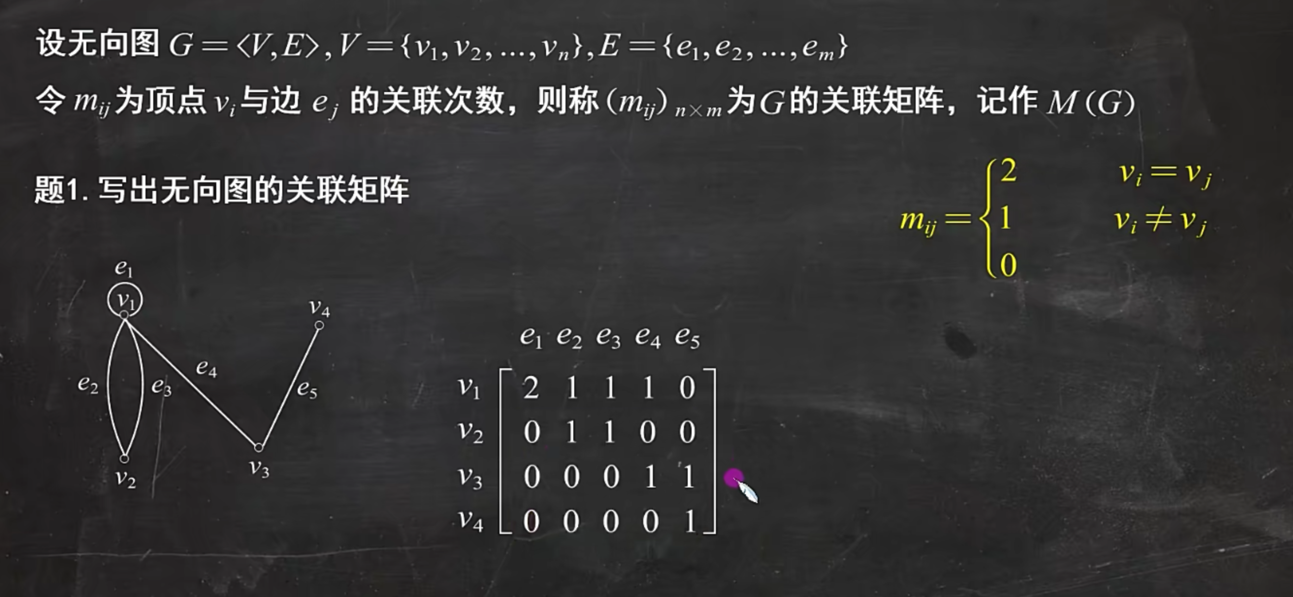
Matrix Representation of Undirected Graphs

The number of rows equals the number of vertices, and the number of columns equals the number of edges.

Matrix Representation of Directed Graphs

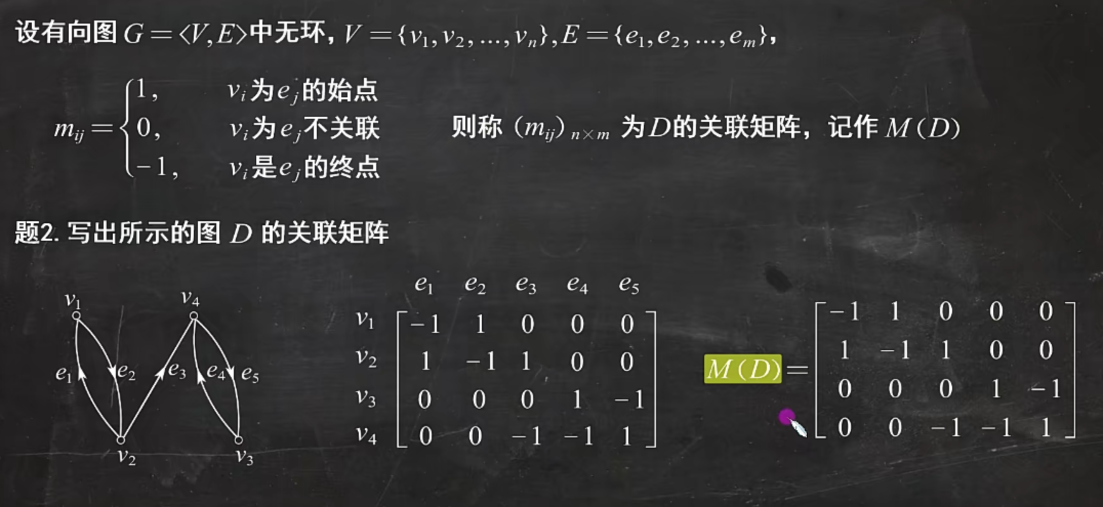
Adjacency Matrix

Mathematical Induction

Steps of Mathematical Induction

1. Base Step:

   • Prove that the proposition holds for the first value (usually n=1).

2. Inductive Step:

   • Assume the proposition holds for some value k, i.e., assume the proposition is true for n=k.
   • Under this assumption, prove that the proposition also holds for n=k+1.

If both steps are completed, then by mathematical induction, the proposition holds for all positive integers n.

Summary of Problem-Solving Steps

1. Base Step: Verify whether the proposition holds when n=1.
2. Inductive Hypothesis: Assume the proposition holds when n=k.
3. Inductive Step: Under the inductive hypothesis, prove that the proposition also holds when n=k+1.

Example: Prove 1 + 2 + 3 + ... + n = n(n+1)/2

Base Step

We first prove that the proposition holds when n=1.

Left side: 1

Right side: 1(1+1)/2 = 2/2 = 1

The left side equals the right side, so the proposition holds when n=1.

Inductive Step

Assume the proposition holds when n=k, i.e., assume: $1 + 2 + 3 + \cdots + k = \frac{k(k+1)}{2}$

Under this assumption, we need to prove that the proposition also holds when n=k+1. That is, we need to prove: $1 + 2 + 3 + \cdots + k + (k+1) = \frac{(k+1)((k+1)+1)}{2}$

By the inductive hypothesis, the left side can be written as: $\left(1 + 2 + 3 + \cdots + k\right) + (k+1) = \frac{k(k+1)}{2} + (k+1)$

Let's simplify the right side: $\frac{k(k+1)}{2} + (k+1) = \frac{k(k+1) + 2(k+1)}{2} = \frac{(k+1)(k+2)}{2}$

This is exactly the right side form we need to prove: $\frac{(k+1)((k+1)+1)}{2}$

Therefore, the inductive step is also complete.

Inclusion-Exclusion Principle

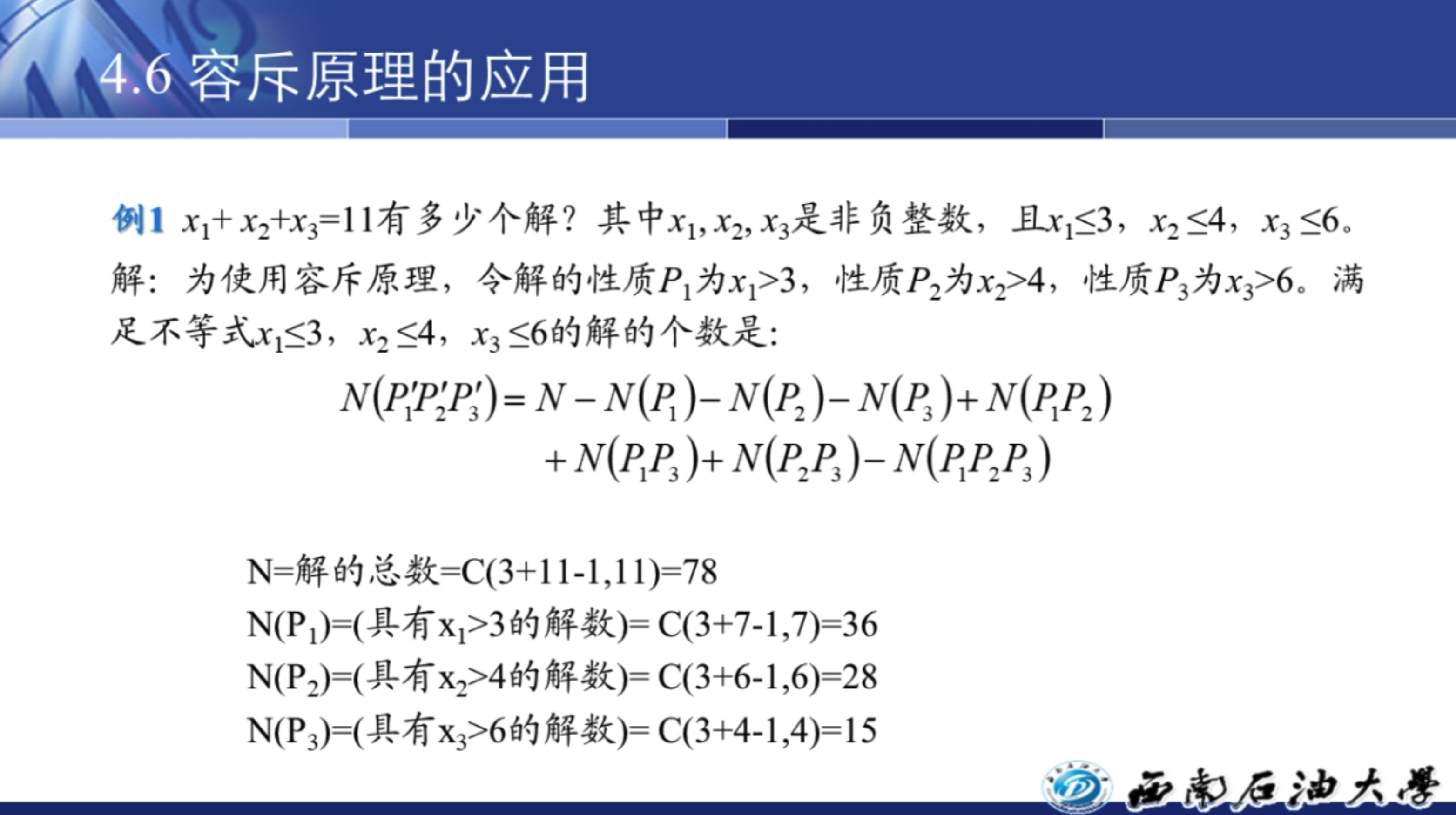
Our problem is to find the non-negative integer solutions to the equation x₁ + x₂ + x₃ = 11. Here we do not consider any constraints. This problem can be transformed into the "stars and bars" method in combinatorics.

Stars and Bars Explanation

To divide 11 units into 3 groups, we can use 2 dividers to split 11 units into 3 parts. Therefore, the problem transforms into inserting 2 dividers among 11 units.

For example, 11 units can be represented as: • • • • • • • • • • •

We need to insert 2 dividers among these units. For instance, inserting them after the 4th and 8th units gives: • • • • | • • • • | • • •

This divides the 11 units into three parts, each representing the values of x₁, x₂, and x₃.

Mathematical Formula Derivation

The above problem is equivalent to choosing 2 positions among 11 units to place dividers. This is a combination problem with the formula:

$$N = \binom{n + r - 1}{r - 1}$$

where n is the number of units and r is the number of variables. For our example:

• n = 11 (total units)
• r = 3 (number of variables)

So we need to calculate:

$$N = \binom{11 + 3 - 1}{3 - 1} = \binom{13}{2}$$

Calculating the Combination

The formula for calculating the combination C(13,2) is:

$$\binom{13}{2} = \frac{13!}{2!(13-2)!} = \frac{13 \times 12}{2 \times 1} = 78$$

Therefore, the total number of non-negative integer solutions N is 78.

Solution

First, the problem asks how many non-negative integer solutions exist for x₁ + x₂ + x₃ = 11, where x₁ ≤ 3, x₂ ≤ 4, x₃ ≤ 6.

Using the inclusion-exclusion principle, let:

• Property P₁ be x₁ > 3
• Property P₂ be x₂ > 4
• Property P₃ be x₃ > 6

To calculate the number of solutions satisfying these inequality constraints, use the inclusion-exclusion formula:

N(P₁'P₂'P₃') = N - N(P₁) - N(P₂) - N(P₃) + N(P₁P₂) + N(P₁P₃) + N(P₂P₃) - N(P₁P₂P₃)

where N is the total number of non-negative integer solutions without considering constraints:

N = C(3+11-1, 11) = C(13, 11) = 78

Next, we focus on explaining how to find N(P₁), i.e., the number of solutions where x₁ > 3:

Finding N(P₁)

The condition x₁ > 3 means x₁ is at least 4. Therefore, we set x₁' = x₁ - 4, so x₁' ≥ 0.

After replacing x₁ with x₁', the original equation becomes: x₁' + 4 + x₂ + x₃ = 11, which simplifies to x₁' + x₂ + x₃ = 7.

Now the problem becomes finding the number of non-negative integer solutions for x₁' + x₂ + x₃ = 7.

The number of solutions for this problem is: N(P₁) = C(3+7-1, 7) = C(9, 7) = 36

Similarly, Finding N(P₂) and N(P₃)

• N(P₂) corresponds to x₂ > 4. Setting x₂' = x₂ - 5, we need to find solutions for x₁ + x₂' + x₃ = 6: N(P₂) = C(3+6-1, 6) = C(8, 6) = 28

• N(P₃) corresponds to x₃ > 6. Setting x₃' = x₃ - 7, we need to find solutions for x₁ + x₂ + x₃' = 4: N(P₃) = C(3+4-1, 4) = C(6, 4) = 15

Using Inclusion-Exclusion to Find the Final Result

Substituting all N(P₁), N(P₂), N(P₃), and their combinations into the inclusion-exclusion formula to calculate the final result:

N(P₁'P₂'P₃') = 78 - 36 - 28 - 15 + N(P₁P₂) + N(P₁P₃) + N(P₂P₃) - N(P₁P₂P₃)

The methods for finding N(P₁P₂), N(P₁P₃), N(P₂P₃), and N(P₁P₂P₃) are similar to the above, except the right side of the equation decreases further.

Recurrence Relations

Below is a detailed explanation of the steps for solving recurrence relations, formatted in LaTeX.

1. Write the Recurrence Relation

The given recurrence relation is: $a_n = -5a_{n-1} - 6a_{n-2} + 42 \cdot 4^n$

2. Determine the Characteristic Equation

To solve the homogeneous part, we first ignore the non-homogeneous term to obtain the corresponding homogeneous recurrence relation: $a_n^{(h)} = -5a_{n-1} - 6a_{n-2}$

Write the characteristic equation. Assuming $a_n^{(h)} = r^n$, substitute into the homogeneous recurrence relation: $r^n = -5r^{n-1} - 6r^{n-2}$

Divide both sides by $r^{n-2}$: $r^2 = -5r - 6$

Obtain the characteristic equation: $r^2 + 5r + 6 = 0$

3. Solve the Characteristic Equation

Solve the characteristic equation: $r^2 + 5r + 6 = 0$

Using the quadratic formula $r = \frac{-b \pm \sqrt{b^2 - 4ac}}{2a}$, where a = 1, b = 5, c = 6: $r = \frac{-5 \pm \sqrt{25 - 24}}{2}$ $r = \frac{-5 \pm 1}{2}$

Obtain two roots: $r_1 = -2, \quad r_2 = -3$

4. General Solution of the Homogeneous Part

Since the characteristic equation has two distinct real roots -2 and -3, the general solution of the homogeneous part is: $a_n^{(h)} = \alpha(-2)^n + \beta(-3)^n$ where α and β are undetermined constants.

5. Find the Particular Solution

Now find the particular solution for the non-homogeneous part. The non-homogeneous term is 42 · 4ⁿ. We assume the particular solution has the form: $a_n^{(p)} = c \cdot 4^n$

6. Substitute into the Original Recurrence Relation to Find the Particular Solution

Substitute the assumed particular solution into the original recurrence relation: $c \cdot 4^n = -5c \cdot 4^{n-1} - 6c \cdot 4^{n-2} + 42 \cdot 4^n$

Divide both sides by 4ⁿ⁻²: $16c = -20c - 6c + 672$

Solve this equation: $16c = -26c + 672$ $42c = 672$ $c = 16$

Therefore, the particular solution is: $a_n^{(p)} = 16 \cdot 4^n$

7. General Solution of the Original Recurrence Relation

The total solution is the sum of the homogeneous solution and the particular solution: $a_n = a_n^{(h)} + a_n^{(p)}$ $a_n = \alpha(-2)^n + \beta(-3)^n + 16 \cdot 4^n$

8. Use Initial Conditions to Find Constants

Use the initial conditions a₁ = 56 and a₂ = 278 to solve for α and β.

For n = 1: $56 = \alpha(-2) + \beta(-3) + 16 \cdot 4$ $56 = -2\alpha - 3\beta + 64$ $-2\alpha - 3\beta = -8 \quad \text{(1)}$

For n = 2: $278 = \alpha(-2)^2 + \beta(-3)^2 + 16 \cdot 4^2$ $278 = 4\alpha + 9\beta + 256$ $4\alpha + 9\beta = 22 \quad \text{(2)}$

Solve the system of equations (1) and (2): $-2\alpha - 3\beta = -8$ $4\alpha + 9\beta = 22$

First solve the first equation: $-6\alpha - 9\beta = -24 \quad \text{(3)}$ Then add (3) and (2): $4\alpha + 9\beta + (-6\alpha - 9\beta) = 22 - 24$ $-2\alpha = -2$ $\alpha = 1$

Substitute into equation (1) to find β: $-2(1) - 3\beta = -8$ $-2 - 3\beta = -8$ $3\beta = 6$ $\beta = 2$

9. Final Solution

Substituting the values of α and β: $a_n = (-2)^n + 2(-3)^n + 16 \cdot 4^n$

Through the above detailed steps, we have successfully solved the recurrence relation. In summary.

Transitive Closure Algorithm Based on Powers

The transitive closure algorithm based on 0-1 matrix powers is a method for computing the transitive closure of a relation. The transitive closure means that if there exists a path from element a to element b in a relation, then the transitive closure relation also contains a direct relation from a to b. The method based on 0-1 matrix powers uses matrix multiplication to compute the transitive closure.

Specific Algorithm Steps:

1. Initialize the Matrix:

   • First, represent the relation R as a 0-1 matrix A. For the set $\{a, b, c, d, e\}$, the size of matrix A is 5 × 5.
   • If (a, b) ∈ R, then the corresponding element in A is 1; otherwise, it is 0.

2. Calculate Matrix Powers:

   • Calculate the power matrices A², A³, ..., Aⁿ until the matrix no longer changes. Matrix power calculation uses Boolean multiplication, where 1 × 1 = 1 and 0 × anything = 0.

3. Calculate the Transitive Closure:

   • The transitive closure matrix B can be obtained by performing an OR operation on all power matrices, i.e., B = A ∨ A² ∨ A³ ∨ ... ∨ Aⁿ.

Example Calculation:

Given the set $\{a, b, c, d, e\}$ and the relation $R = \{ (a, c), (b, d), (c, a), (d, b), (e, d) \}$, first convert it to a 0-1 matrix A:

$$A = \begin{pmatrix} 0 & 0 & 1 & 0 & 0 \\ 0 & 0 & 0 & 1 & 0 \\ 1 & 0 & 0 & 0 & 0 \\ 0 & 1 & 0 & 0 & 0 \\ 0 & 0 & 0 & 1 & 0 \end{pmatrix}$$

Next, calculate the power matrices of A:

$$A^2 = A \times A = \begin{pmatrix} 1 & 0 & 0 & 0 & 0 \\ 0 & 1 & 0 & 0 & 0 \\ 0 & 0 & 1 & 0 & 0 \\ 0 & 0 & 0 & 1 & 0 \\ 0 & 1 & 0 & 0 & 0 \end{pmatrix}$$ $$A^3 = A \times A^2 = A = \begin{pmatrix} 0 & 0 & 1 & 0 & 0 \\ 0 & 0 & 0 & 1 & 0 \\ 1 & 0 & 0 & 0 & 0 \\ 0 & 1 & 0 & 0 & 0 \\ 0 & 0 & 0 & 1 & 0 \end{pmatrix}$$

Since A⁴ = A² and A⁵ = A³, we can stop calculating.

Finally, calculate the transitive closure matrix B:

$$B = A \lor A^2 = \begin{pmatrix} 1 & 0 & 1 & 0 & 0 \\ 0 & 1 & 0 & 1 & 0 \\ 1 & 0 & 1 & 0 & 0 \\ 0 & 1 & 0 & 1 & 0 \\ 0 & 1 & 0 & 1 & 0 \end{pmatrix}$$

Therefore, the 0-1 matrix B of the transitive closure of relation R is:

$$B = \begin{pmatrix} 1 & 0 & 1 & 0 & 0 \\ 0 & 1 & 0 & 1 & 0 \\ 1 & 0 & 1 & 0 & 0 \\ 0 & 1 & 0 & 1 & 0 \\ 0 & 1 & 0 & 1 & 0 \end{pmatrix}$$

Through the above steps, we can obtain the 0-1 matrix of the transitive closure of relation R.

Transitive Closure Error Problem

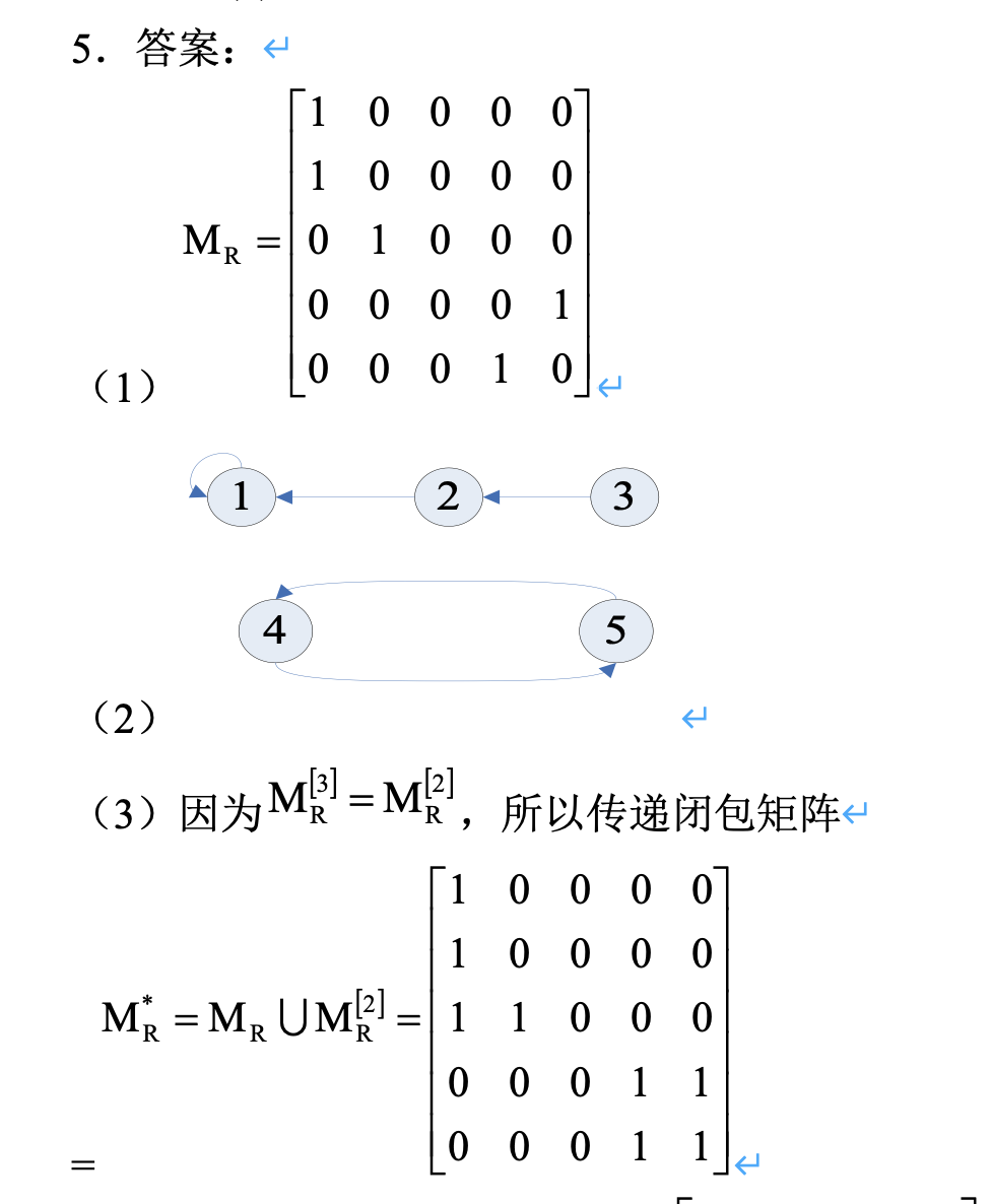
Note that vertices 4 and 5 have paths to each other. When computing the transitive closure, (5,5) and (4,4) should be included.

Equivalence Classes

An equivalence class is a set of elements that are equivalent under an equivalence relation. Under an equivalence relation $R$, given an element $a \in A$, its equivalence class $[a]_R$ is the set of all elements equivalent to $a$. Formally:

$[a]_R = \{x \in A \mid (a,x) \in R\}$

Let's look at the specific equivalence relation R in the problem:

Set $A = \{a, b, c, d, e, f\}$, and the equivalence relation $R$ is:

$$R = \{ (a,a), (b,b), (c,c), (a,b), (b,a), (a,c), (c,a), (b,c), (c,b), (d,d), (e,e), (d,e), (e,d), (f,f) \}$$

To find $[a]_R$, we need to find all elements equivalent to $a$. According to the definition of $R$, we can see:

$$(a,a), (a,b), (a,c), (b,a), (c,a)$$

So, the elements equivalent to a are: a, b, c.

Therefore, $[a]_R = \{a, b, c\}$.

In summary:

$$[a]_R = \{a, b, c\}$$

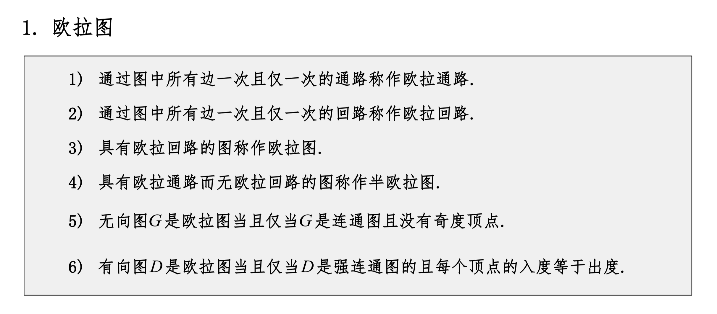
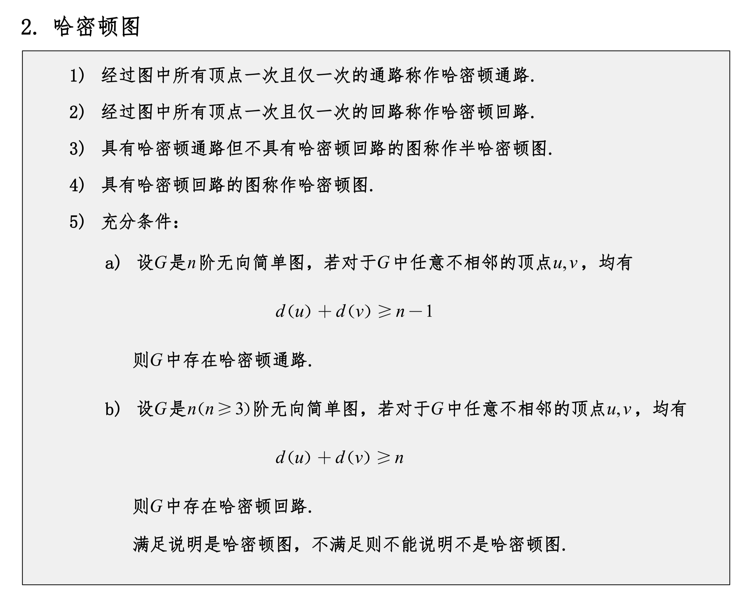
Euler Graphs, Hamiltonian Graphs